
Software Resources | fMRI Lab

Luis' Shared Code
Ortho, f-ASL
This page contains some of the programs Luis Hernandez-Garcia has written over the last few years at the University of Michigan, which he often uses in his work. Hernandez-Garcia is happy to share his work with others, but asks that you email him if you download the programs so he knows whether the material is useful. You can modify anything you want to suit your needs.
DISCLAIMER from Hernandez-Garcia: I am not responsible for what happens to your data. Just because it works for me doesn't mean that it will work for you. That said, please let me know if you find any bugs. Chances are, you will find quirks here and there. Please send me an email if you find bugs, and I'll see what I can do!
Luis' Tools
Both programs described here are bundled in a single tar file. Download the whole Toolbox.
Installation
This TAR file contains several tools for displaying and analyzing images in MATLAB. There are many interdependencies among the functions, so I recommend downloading the entire toolbox to avoid issues. Some of these functions also use SPM functions.
Download the .tar file (LuisTools.tar) and extract it to a directory of your choice.
tar xvf LuisTools.tar
Add that directory to your MATLAB path. For instructions on how to use a specific function from the toolbox, say, "blah.m", simply type (within MATLAB)
> help blah
You will get instructions on using input and output.
f-ASL
An interactive tool for analysis of arterial spin labeling functional MRI time series data. It includes preprocessing, physiological noise correction, OLS and GLS analyses, and quantification of perfusion.
Brief User Manual (f-ASL)
To start f-ASL, run MATLAB and execute the command:
fasl01
A GUI interface will pop up. The general idea is to provide a raw data file and check everything you want to do with the data. When you click GO, the program will execute the options you checked in order from top to bottom. It’s really simple.
If you plan to perform a GLM analysis, you will need to load a design matrix from a text file. If you don't already have one, click the "Build Design Matrix" option to generate it. The ASL design matrix builder tool will open, and you can fill in the regressors one by one.
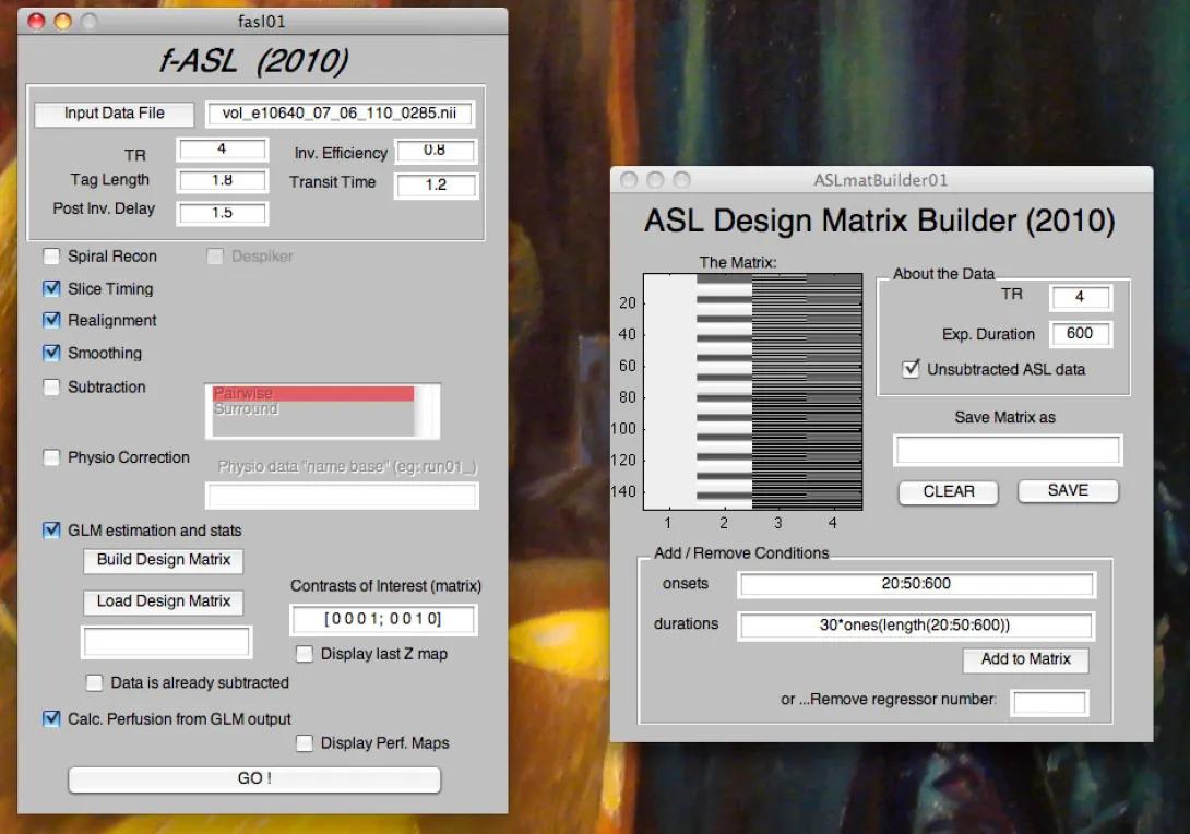
Screenshot of two application windows related to arterial spin labeling analysis. The left window, titled “f-ASL (2010),” shows fields for input data file, TR, tag length, inversion efficiency, transit time and post-inversion delay, along with checkboxes for processing steps such as slice timing, realignment, smoothing and GLM estimation. The right window, titled “ASL Design Matrix Builder (2010),” displays a grayscale design matrix plot, fields for TR and experiment duration, options for unsubtracted ASL data and controls to add or remove regressors.
Program Features
- It has a tool for physiological noise correction using RETROICOR, adapted for ASL data
- It creates the design matrix for unsubtracted ASL data for you.
If analyzing unsubtracted data, the program will do GLS estimation (prewhitening of the data).
See: Mumford, J.A., Hernandez-Garcia, L., Lee, G.R., Nichols, T.E., 2006. Estimation efficiency and statistical power in arterial spin labeling fMRI. Neuroimage 33, 103-114.
After GLM estimation, it converts parameter estimates into meaningful perfusion effects in units of perfusion (ml/min/100g). Please see the forthcoming paper (you can already see it in PubMed, though):
Hernandez-Garcia L, Jahanian H, Rowe DB: Quantitative Analysis of Arterial Spin Labeling FMRI Data Using a General Linear Model. Magnetic Resonance Imaging, 28 (7), Pages 919-927, 2010. [PMID: 20456889]
If you know how to program MATLAB, you can run it in a batch mode (skipping the GUI) by calling the "master program" from a script. FASL is just a nice GUI wrapper around this other program. The program file is asl_spm01.m. To use it, all you have to do is update the contents of the structure "args" and call
asl_spm01(args)
Type help asl_spm01 to get a complete listing of the contents of "args" and how to use it.
Important Notes
- Some things are hard-coded, and you may need to get under the hood or contact me about how to change them. IN particular, the physio correction process is tailored to our scanner's sampling rate and our naming scheme for the physiological data files. Right now, you need to get into the code and edit it to change that. Not being familiar with many scanners, I’m not sure how to do a generic one. In the meantime, you can email me, and I'll help.
- The reconstruction code is also set up to reconstruct images from our scanner and our specific pulse sequence, so you'll want to skip that part and start out with already reconstructed images from your site. If you're a regular MATLAB hacker, it should be easy to stick in your own reconstruction code into it.
- The slice timing correction interpolates the data to the last slice in the acquisition. Make sure you know your acquisition timing parameters.
- The smoothing tool is set to use a Gaussian kernel with a 3-voxel width.
- The realignment is done by SPM 5, and the data gets resliced.
- The quantification model assumes you are running a continuous ASL scheme, such as pseudo-CASL.
Ortho
An interactive tool for visualization and ROI analysis of fMRI time series data. This tool also includes Granger Causality Analysis (use at your own risk).
Brief User Manual (Ortho)
Starting Ortho
Run MATLAB and execute the command:
ortho
(The GUI portion does not work with prior versions of MATLAB 7, but you can still run ortho as a command line tool, though!)
If you want to run ortho without the GUI, take a look at the file ortho_nogui.m. You can edit that file by filling in the fields that you need, and use it as a "fake GUI". Once you have filled it in, all you have to do is execute it.
Similarly, if you want to use the programs in batch mode to run through all your subjects, edit the file ortho_batch.m and execute it.
But if you are one of the lucky ones with MATLAB 7 or later and you are using the GUI, the interface looks like the picture on the right.
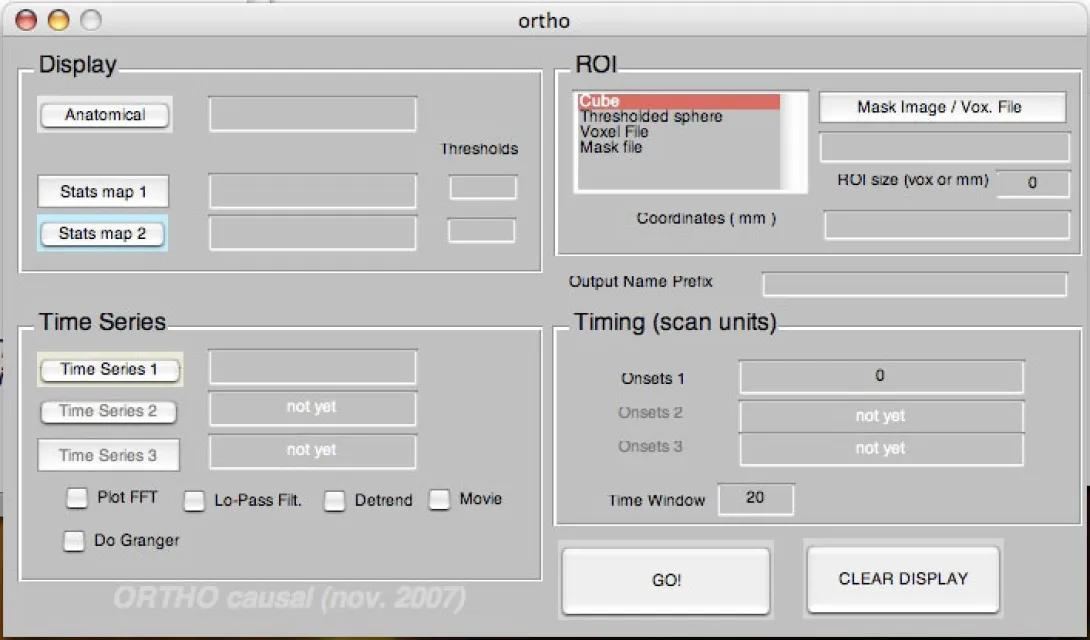
Screenshot of a macOS application window titled “ortho,” showing a gray graphical interface for neuroimaging analysis. The layout includes sections labeled Display, ROI and Time Series. The Display panel has buttons for Anatomical, Stats map 1 and Stats map 2 with threshold fields. The ROI panel lists options such as Cube, Thresholded sphere, Voxel File and Mask file, with fields for mask image, ROI size and coordinates in millimeters. The Time Series panel includes buttons for up to three time series, options like Plot FFT, Lo-Pass Filt., Detrend, Movie and Do Granger, and timing controls for onsets and time window. Large buttons labeled GO! and CLEAR DISPLAY appear at the bottom. The footer reads “ORTHO causal (nov. 2007).”
Using Ortho
Ortho works on Analyze format files (.img) and NIFTI (.nii, .nii.gz). Please note that ORTHO ignores the .mat files generated by SPM. It does use header information, such as origins, voxel sizes and the Scaling Factor.
Now that ORTHO is running, its main functions are to
- Display the images in orthogonal views,
- Overlay statistical maps on top of them, and
- Extract time series from selected voxels. You can easily select the type or ROI you want.
- Show you the pixel values of the anatomical and the statistical images.
ORTHO can also (if you check the options)
- Average events from a time series
- Show you a movie of the image in orthogonal sections.
- Filter the data,
- Display the temporal frequency content. The user can navigate the images interactively, and ORTHO updates the time-series display accordingly.
- Save the time-series data to ASCII files.
- Ortho is VERY easy to run as a batch script. Type " help ortho2005 " at the MATLAB command prompt for details.
Ortho's interface is designed so that when you press the GO button, it displays as much as possible based on the fields the user has filled in (though some combinations are not implemented yet). ORTHO displays the images and updates the display interactively as you select voxels by clicking them. Information about the pixel (or pixels) is displayed in the MATLAB Command Window. When you RIGHT-CLICK, all that information gets put into ASCII files.
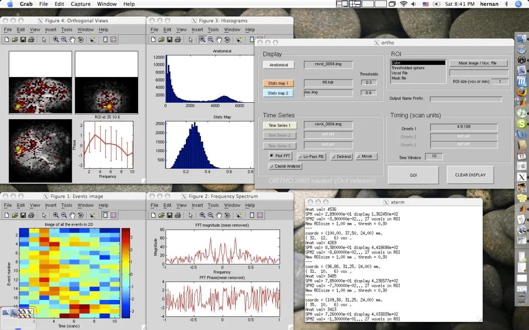
Screenshot showing multiple overlapping neuroimaging analysis windows. The main window, titled “ortho,” displays panels for Anatomical images, Stats map 1 and Stats map 2 with threshold values, ROI options such as Cube and Thresholded sphere, time series controls and timing fields with onsets and time window. Surrounding it are additional figure windows labeled “Orthogonal Views,” “Histograms,” “Events image,” and “Frequency Spectrum,” showing brain slice images with highlighted activation clusters, histograms of anatomical and statistical maps, a color-coded event matrix and FFT magnitude and phase plots. An xterm terminal window on the right lists coordinate values and ROI statistics.
How to do a few basic things using the GUI
Extracting and Looking at a Time Series.
If you fill in the "time series" only, you will get a plot of the time series at whatever voxel you click on. To fill in the "Time Series" field, select one of the images in the time series. ORTHO will assume that they are all named the same except for the numbers at the end of the name. eg-
vol_e2343_10_12_03_0001.img
vol_e2343_10_12_03_0002.img
...etcIf you have a single 4D file, ORTHO will recognize it and read it in as well. If you fill in the "anatomical" image only, you will get a display of the image you select, along with a nice histogram of the pixel values.
Stuff you can do to the time series.
You can also add detrending (3rd-order polynomial) and Gaussian filtering to the time series by checking the appropriate boxes. The filter parameters are hard-coded. They should be user-defined, but that's not implemented yet... sorry... It's easy to hack if you have the inclination, though...
If you click with the RIGHT mouse button, the extracted waveforms get stored as ASCII files for easy access outside of MATLAB.
You can display the FFT's magnitude and phase in a separate window by checking the "FFT" box (near the bottom)
If you provide a set of onset times and a time window, you will get trial averages within that window. Note: Ortho measures time in scans; it does not know your sampling rate or TR. It also displays a clear image of a matrix of the individual events you are averaging. This is really handy because you can notice changes in the events from trial to trial, things like habituation or drifts in HRF parameters, errors in the timing of the experiment...
You can also look at a movie of the time series through the selected location by checking the "Movie" checkbox
Ovelaying a Statistical Map.
If you fill in "anatomical" and "stats map 1", you will see the anatomical image with the statistical map overlaid. You can set the threshold by entering a value in the threshold field. These images must be coregistered previously. They can have different resolutions, but they must be in the same orientation and share the same origin. Remember that ORTHO does not use the .mat files generated by SPM's coregistration, so it doesn't apply transformations on the fly as SPM does.
You can also display two statistical maps to find overlapping voxels by filling in "stats map 2". Overlapping pixels in the statistical maps are shown in green.
You can change the threshold interactively by entering a new value in the interface and clicking a pixel to update the display.
Selecting ROI types.
If you fill in the "Anatomical", "Stats Maps" and "Time Series", you can also select a specific set of voxels to extract the information from. The values in those voxels are averaged. You can choose what kind of ROI to use in the upper right side of the interface:
- Cube means that you get the voxel you click on plus the number of neighbors in each direction specified in the "ROI size" field. The default is a cube with zero neighbors.
- Thresholded Sphere: means a sphere with the radius in mm specified in the field labeled ROI size.
- Mask File: means an Analyze format image in which the voxels of interest have value 1. All others have a value of zero.
- Voxel File means that the ROI consists of a list of voxels specified in an ASCII file, which you have to select by clicking the "Mask File / Vox. File" Button, or just typing in the file name in the field below that button. About the aforementioned voxel file, it needs to be an ascii (text) file that looks like this example:
12 43 45
12 44 46
23 45 89
...etc.Those coordinates are in voxel units, and they are relative to the first voxel in the file - the one in the lower left corner, NOT the origin!
Computing Granger Causality Maps.
There is a CheckBox at the bottom of the GUI that says "Do Granger". IF this is checked, as soon as you right-click on a pixel, the program will compute the Granger Causality F score between the current ROI and the rest of the image. The resulting files are named:
grangerFab - F score of the influence of seed on each voxel
grangerFba - F score of the influence of each voxel on the seed.
grangerF - difference between the two above: a measure of the directionality of the relationship. If it's positive, it means that the seed granger-Causes the voxel in question.
grangerlog10P - a p-value associated with the F score above (I'm not very confident in this p-value computation, though)You also get histograms of the different outputs.
Be careful with Granger Causality; Whether it’s appropriate for BOLD time series data is not clear at all!
