Michigan Model for Diabetes

Modeling Diabetes Progression
A computerized disease model that enables the user to simulate the progression over time of diabetes.
New Models
Explore the newest versions of the model on GitHub.
The Michigan Model for Diabetes (MMD) is a computerized disease model that enables the user to simulate the progression over time of diabetes, its complications (retinopathy, neuropathy and nephropathy), and its major comorbidities (cardiovascular and cerebrovascular disease), and death.
Transition probabilities can be a function of individual characteristics, current disease states or treatment status. The model also estimates the medical costs of diabetes and its comorbidities, as well as the quality of life related to the current health state of the subject.
Contact
If you have any questions/issues please contact us at [email protected].
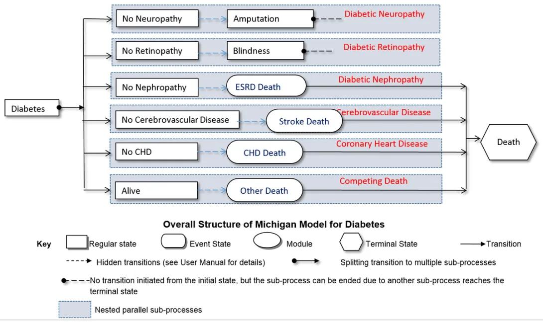
The model depicts the progression of diabetes and associated complications, from initial diagnosis to various end-stage conditions.
The "Overall Structure of Michigan Model for Diabetes" shows the splitting transition to multiple sub-processes from Diabetes and potential complications.
Nested parallel sub-processes include:
1. No Neuropathy (Regular State) has a hidden transition to Amputation (Regular State) with no transition initiated from the initial state, but the sub-process can be ended due to another sub-process that reaches the terminal state of Diabetic Neuropathy.
2. No Retinopathy (Regular State) has a hidden transition to Blindness (Regular State) with no transition initiated from the initial state, but the sub-process can be ended due to another sub-process that reaches the terminal state of Diabetic Retinopathy.
3. No Nephropathy (Regular State) has a hidden transition to ESRD Death (Event State) with a transition to Diabetic Nephropathy and a transition to a terminal state of death.
4. No Cerebrovascular Disease (Regular State) has a hidden transition to Stroke Death (Event State) with a transition to Cerebrovascular Disease and a terminal state of death.
5. No CHD (Regular State) has a hidden transition to CHD Death (Event State) with a transition to Coronary Heart Disease and a terminal state of death.
6. Alive (Regular State) has a hidden transition to other death (Event State) with a transition to competing death and a terminal state of death.
For each subject, the model software reads in or simulates the subject’s baseline characteristics and then advances the subject through a specific number of years or until death. Each year, the model updates in the four stages as indicated by blue blocks in the following graph:
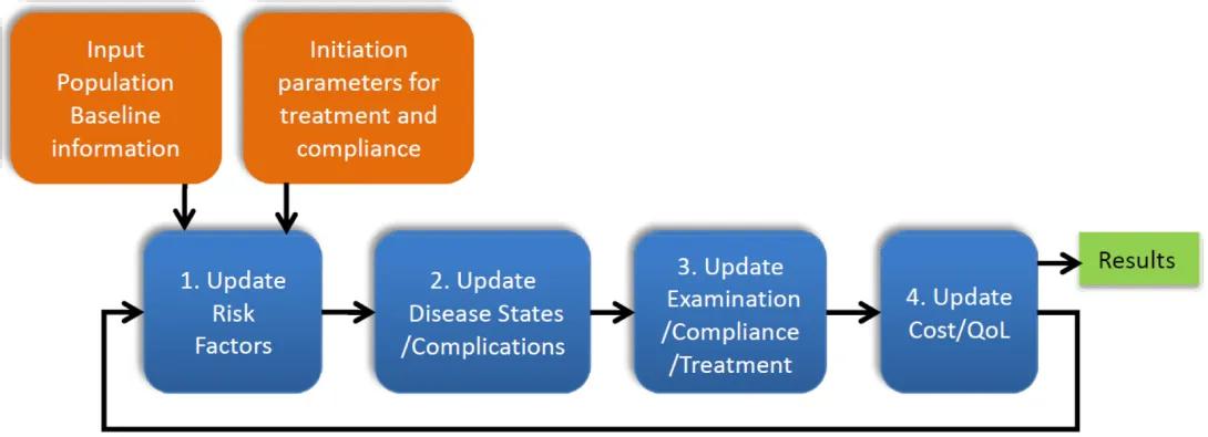
A systematic approach to updating risk factors, disease states, and treatment compliance.
Input Population Baseline Information and Initiation Parameters for Treatment and Compliance lead to:
1. Update Risk Factors
2. Update Disease
3. Update Examination/Compliance/Treatment
4. Update Cost/QoL
The four steps in the process loop and eventually lead to Results.
In contrast to other proposed models, the transition probabilities implemented in the MMD were obtained by synthesizing the published literature. Specifically, transition probabilities in the newly updated coronary heart disease model that reflect the direct effects of medical therapies on outcomes were derived from the literature and calibrated to recently published population-based epidemiologic studies and randomized controlled clinical trials. This method not only allowed us to build a model without access to individual-level data from a long-term prospective study, but allowed us to update the model by incorporating data from new studies as they become available.
In addition, different from other proposed models, our model allows the user to control risk factor changes through defining treatment threshold and compliance rates for dysglycemia, dyslipidemia, and hypertension, and compliance to quitting smoking and taking aspirin. Given the fact that modern medicines have largely decreased the complication rate in type 2 diabetes through management of these risk factors, it is important to explicitly model these management strategies and allow the user to modify them to match the specific scenario that they are simulating. For example, MMD explicitly models the treatment regimen for hyperglycemia through five treatment stages. The following figure shows a mock trajectory of A1c over time under this treatment regimen using 7% as the treatment threshold.
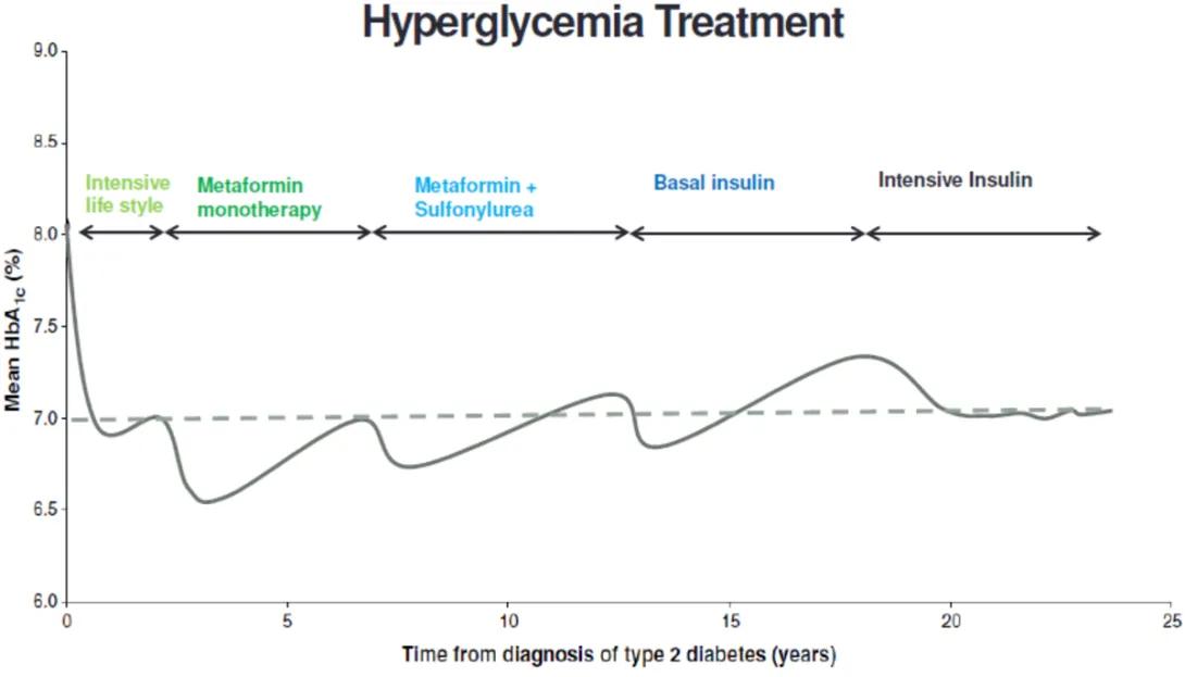
Visual representation of mean HbA1c response to intensive lifestyle, metformin monotherapy, metformin plus sulfonylurea, basal insulin, and intensive insulin over time.
The graph for "Hyperglycemia Treatment" depicts the progression of mean HbA1c (%) levels over time from the diagnosis of type 2 diabetes. The x-axis represents the time from diagnosis in years, ranging from 0 to 25 years, and the y-axis shows mean HbA1c (%) levels, ranging from 6.0% to 9.0%. There is a dashed horizontal line at 7.0%.
There are four phases of treatment noted on the graph, with corresponding fluctuating lines showing how mean HbA1c levels change with each treatment:
1. Intensive Lifestyle: Initially after diagnosis, there's a sharp decline in HbA1c levels.
2. Metformin Monotherapy: After the initial decline, HbA1c levels begin to rise gradually.
3. Metformin + Sulfonylurea: This phase starts around the time when HbA1c levels are approximately at the 7.0% threshold before they begin to rise again.
4. Basal Insulin: After some years, HbA1c levels increase over 7%.
5. Intensive Insulin: Eventually, HbA1c levels plateau around 7%, signaling this final treatment phase.
The following two figures show how A1c and SBP change over time in a simulated population.
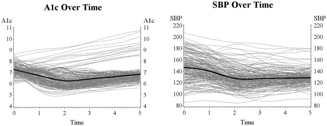
Visualizing the average A1c and SBP levels over time, with individual data points included.
The left line graph, titled "A1c Over Time," shows the trend of A1c levels over a period of 5 time units, presumably years or months. The A1c levels on the y-axis range from 4 to 11. Multiple fine gray lines represent individual trajectories, and a bold black line indicates the average trend. The graph shows a general decline in A1c levels, starting from a level slightly above 7, reaching a low point around 6, and then slightly increasing beyond 3 time units.
The right graph, titled "SBP Over Time," depicts the change in SBP (Systolic Blood Pressure) over the same time span. The SBP levels on the y-axis range from 80 to 220. Similar to the left graph, numerous fine gray lines signify individual SBP trends, with a bold black line representing the average trend. The overall pattern shows a decrease in SBP from around 145 to slightly above 125 and then stabilizes after 3 time units.
The updated coronary sub-model has been internally and externally validated. Panel A shows the results of internal validation. Panel B shows the results of external validation. The MMD group continues to extend the external validation against the latest clinical and epidemiological data.
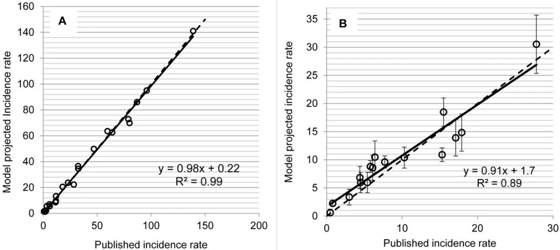
Model A demonstrates a high degree of accuracy (R² = 0.99) in predicting incidence rates.
Model B shows a strong positive correlation (R² = 0.89) between published and projected incidence rates.
The image consists of two scatter plots, labeled A and B, comparing model-projected incidence rates with published incidence rates.
- Panel A: This scatter plot shows a series of data points plotted along a linear regression line comparing the model-projected incidence rate (y-axis) to the published incidence rate (x-axis) with values ranging from 0 to 200. The equation for the best-fit line is given as y = 0.98x + 0.22, with an R² value of 0.99, indicating a very high degree of correlation between the model projections and the published data. The points closely follow the best-fit line, indicating strong agreement between model predictions and observed data.
- Panel B: This scatter plot has data points along a linear regression line with error bars shown on each point. The x-axis (published incidence rate) ranges from 0 to 30, and the y-axis (model-projected incidence rate) ranges from 0 to 35. The equation for the regression line is y = 0.91x + 1.7, with an R² value of 0.89, suggesting a strong but slightly lesser correlation compared to Panel A. The presence of error bars suggests variability or uncertainty in the measurements, and the points also follow the best-fit line closely, but with more scatter than in Panel A.
MMD is implemented using a general chronic disease modeling software IEST (Indirect Estimation and Simulation Tool) which provides an environment for model design, estimation, and simulation, as well as a convenient graphical user interface to (1) define parameters, (2) define populations, (3) generate populations from distributions, (4) create a new disease model or modify an existing model, (5) simulate the behavior of a given base population by using a defined model enhanced by a set of simulation rules, and (6) analyses and report simulation results. The software is being released for use by researchers under a general public license.
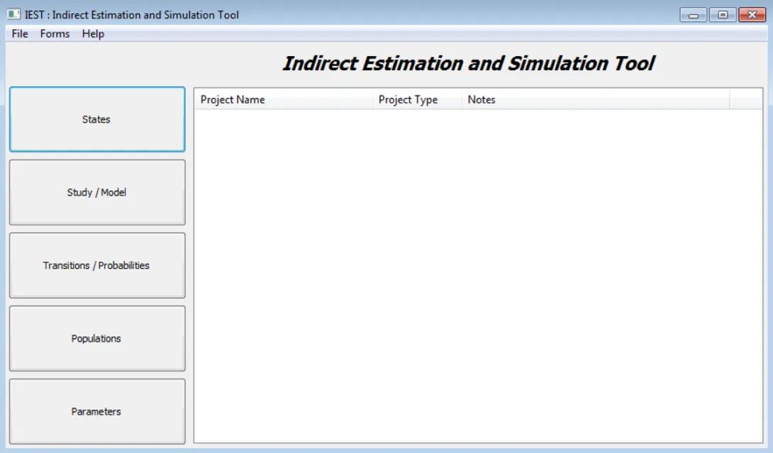
Indirect Estimation and Simulation Tool screen
The image is a screenshot of a software application window titled "Indirect Estimation and Simulation Tool." Below this title, there is a table header with columns labeled "Project Name," "Project Type," and "Notes."
Below the menu, on the left side, there are five large buttons arranged vertically with the following labels: "States," "Study / Model," "Transitions / Probabilities," "Populations," and "Parameters."