IEST Help

Copyright © 2009-2025 The Regents of the University of Michigan. Initially developed by Deanna Isaman, Jacob Barhak, Morton Brown, Wen Ye. Additional coding by Donghee Lee, Ray Lillywhite, Aidan Feldman. Videos by Michael Kylman.

This documentation and software are part of the Indirect Estimation and Simulation Tool (IEST). The Indirect Estimation and Simulation Tool (IEST) is free software: you can redistribute it and/or modify it under the terms of the GNU General Public License as published by the Free Software Foundation, either version 3 of the License, or (at your option) any later version.

The Indirect Estimation and Simulation Tool (IEST) is distributed in the hope that it will be useful, but WITHOUT ANY WARRANTY; without even the implied warranty of MERCHANTABILITY or FITNESS FOR A PARTICULAR PURPOSE. See the GNU General Public License for more details.

Additional Clarification

The Indirect Estimation and Simulation Tool (IEST) is distributed in the hope that it will be useful, but "as is" and WITHOUT ANY WARRANTY of any kind, including any warranty that it will not infringe on any property rights of another party or the IMPLIED WARRANTIES OF MERCHANTABILITY or FITNESS FOR A PARTICULAR PURPOSE. THE UNIVERSITY OF MICHIGAN assumes no responsibilities with respect to the use of the Indirect Estimation and Simulation Tool (IEST).

This version of the Indirect Estimation and Simulation Tool enables defining a disease model and using this model for a Monte Carlo simulation of a given population set. It also allows running the estimation model for a single model sub-process using the same estimation technique used by the previously published Matlab Prototype.

This version allows the user to create and run models through a Graphic User Interface (GUI). Yet the system will also capable or running simulations in High Performance Computing (HPC) environment using a computer cluster.

This version also contains fixes to previous versions. See the README.txt file supplied with the software for further information on changes and capabilities.

4. Setup

4.1 Environment

NOTE: This software has been tested on Microsoft Windows XP and Linux. Note that other operating systems (such as OS X and other Windows versions) may work, yet were not fully tested.

Windows

• Python version 2.7, a Python version for Windows can be downloaded from: here. If this link does not work for you, you may find an alternate version by visiting the following webpage: http://python.org/download/releases/2.7.2/
• wxPython (Requires Python), a Unicode version suitable for Python version 2.7 for Windows 32 bit can be downloaded from here. If this link does not work for you, you may find an alternate version by visiting the following webpage: http://www.wxpython.org/download.php#stable
• The NumPy library (Requires Python), a version suitable for Python version 2.7 for Windows can be downloaded from here(link is external). If this link does not work for you, you may find an alternate version by visiting the following webpage: http://www.scipy.org/Download
• The SciPy library (Requires Python and NumPy), a version suitable for Python version 2.7 can be downloaded from here. If this link does not work for you, you may find an alternate version by visiting the following webpage: http://www.scipy.org/Download(The above is an essential list and the software will run with these with diminished capabilities.If you plan to create plots from simulation results, you will also need to install the following:
• The matplotlib library (Requires Python), Version 1.1.0 was used and can be downloaded from here. If this link does not work for you, you may find an alternate version by visiting the following webpage: http://sourceforge.net/projects/matplotlib/files/ If you plan to use estimation capabilities that are typically less in use, you will also need to install the following:
• The Sympy library (Requires Python), Version 0.7.1 was used and can be downloaded from here. If this link does not work for you, you may find an alternate version by visiting the following webpage: http://code.google.com/p/sympy/downloads/list(link is external)

OS X

• Python for OS X is included by default on all OS X installations.
• Install pip to assist with the installation of non-standard Python modules used by the IEST software by visiting the following webpage: http://pip.readthedocs.org/en/latest/installing.html and downloading the "get-pip.py" file. Save the file to your desktop.
• Open the application "Terminal" through Applications -> Utilities -> Terminal and issue the following commands:
  • sudo python ~/Desktop/get-pip.py
  • sudo pip install numpy
  • sudo pip install scipy
• Download wxPython2.8.12 ansi version (NOT unicode like Windows from above) by visting the following webpage, and install the subsequent .dmg file: http://sourceforge.net/projects/wxpython/files/wxPython/2.8.12.1/wxPython2.8-osx-ansi-2.8.12.1-universal-py2.7.dmg/download

4.2 Software Installation

After the environment has been properly installed:

• Using your web browser, access the project web site at the software section here
• Download the archive file InstallIEST###.zip where ### stands for the version of the software. You should use the highest version available.
• Extract the downloaded archive to a directory of your choice. This will be your working directory.
• If using OS X or Linux, Unzip the IEST software and issue the following command in the unzipped IEST working directory:
  • python Main.py

4.3 Running the Software

Open the working directory created during installation and double-click Main.py. The main form of the system, titled 'Indirect Estimation and Simulation Tool', will open. This is further described in the section Getting Started with IEST.

5. Getting Started with IEST

5.1 Running the Software

Open the folder created during installation and double-click Main.py. The form, 'Indirect Estimation and Simulation Tool', will open.

From this form the user can load and save data and access all system parameters. Here is a short description of the basic operations that one can perform with this form:

5.1.1 Handling Data Files

The system holds its data in files in a zip archive. Each file can contain many Projects/Models/Populations using the same or different terminology. The system can load this information and at the end of work the user can save the modified information back to a file. Note that while working with the system the information is never saved to a file until the user specifies the save in this form.

Loading a Data File

1. From the menu bar at the top of the main form, select File.
2. From the File menu select Open.
3. Select the requested filename/path of the data file from the new window that appeared and press the Open Button.
4. The label at the top of the windows should show the path of the file and the project list (A) should show projects held within the loaded file.

Saving a Data File

1. From the menu bar at the top of the main form, select File.
2. From the File menu select Save to save under a default file name. Select Save As to modify filename/path.
3. The label at the top of the windows should show the updated path of the file if this was changed. Note that if a system overwrites an existing file it will maintain a copy of the old file under a file name with an extension of a numerical timestamp representing the time/date of the new file created. This backup file can be loaded into the system.

In the event the system does not close properly any modifications made will be lost. A proper exit of the system will ask the user to save the information to file. The automatic backup mechanism during file saving helps track back changes in data and helps maintain integrity.

Note that the system does not lock files after loading them during work. Also note that saving records in the system is not the same as saving the file. Records and entities in other forms are saved to memory rather than to a file. The only way to save to a file is through the main form menu.
For a video demonstration of loading and saving files, click here.

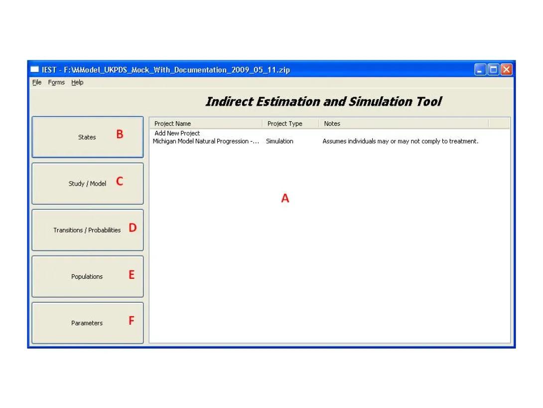
5.1.2 Projects

A project is the main entity defined in the system. Projects can be either Simulation Projects or Estimation Projects. Projects can share information such as models or parameters.

All the projects currently loaded in the system are listed in the main form in the project list (A).

To view a project, double click its entry in the list (A) in the main form. The appropriate form will open.

To add a new project to the system, double click the text Add New Project at the top of the list (A). Then select the type of the project from the window that will open. The appropriate form will open.

Simulation Projects or Estimation Projects will have different forms to handle the information in them. See Simulation/Estimation for additional details.

5.1.3 The First Time Running the System

One way to familiarize yourself with the system is to load the test examples file Testing.Zip created by the system during installation. This file provides an implementation of all the simulation examples provided in the test example document SimulationExamples.pdf that is also created by the installation.

Each project is an example from this document. Double clicking on projects listed in (A) will open the project clicked upon. Clicking the buttons marked as (B,C,D,E,F) will allow exploring the underlying data that created these projects.

5.2 Work Flow with the System

Before working with the computer system, some preparation is required. This page describes the preparation stages and the workflow with the system from a more abstract view.

5.2.1 Literature Review

When developing a new model or modifying an existing model, it is essential to perform an extensive literature review and to consult with clinical experts who can describe the progression of the disease. During the literature review, it is important to identify studies that provide estimates of the transition probabilities for the progression of the disease through time.

5.2.2 Building the Disease Model

Understanding the Disease Structure

The information from the literature review must be translated into system terminology. This involves identification of important keywords that describe disease progression; these are then used in different categories defined by the computer system:

• States - define the condition of the individual
• Sub-process - a collection of states that describe a condition and may consistent of a sequence of several states. Subprocesses may occur in parallel to each other, or may be nested within a different subprocess.
• Parameters - characteristics such as Age, blood pressure, Costs that affect the progression of the disease or change due to its progression.
• Rules - Logic statements that describe changes in the disease or in associated parameters

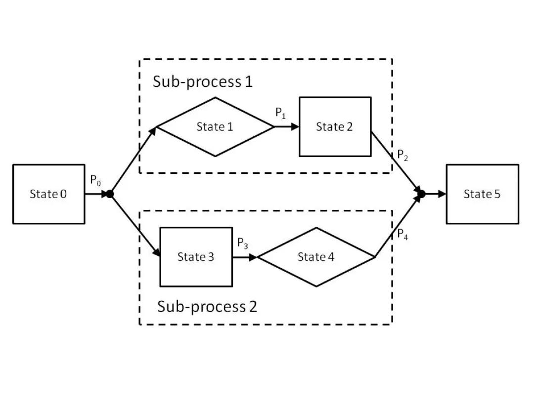
Building the Model Diagram

The identified states and sub-processes should be depicted as boxes in a diagram; the boxes should be connected with arrows to signify transitions between states. Note that at this point, the probabilities of the transitions are considered unknown and denoted by a coefficient. The output of this state may look like:

5.2.3 Estimate the Disease Progression Parameters

See Estimation

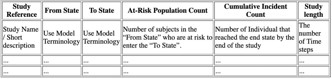
Synthesizing Study Information

The statistical information from the literature review should be extracted into the following table.

Calculating Model Parameters

The study data and the model should be entered into the system. Then, the estimation module should be run and as a result the unknown coefficients in the model will be estimated. With this version estimation should be repeated for each sub-process separately. Afterwards, the simulation model is almost ready.

If the model does not require estimation of parameters from studies, then the model can be entered directly as a simulation model to the system as described in Simulation.

5.2.4 Simulating Disease Progression

See Simulation for details.

Define a Simulation Population Set

It is necessary to specify the population of individuals to whom the simulation should apply. The population should contain information about the initial states of each individual. Also, parameters to be used in the simulation should be defined.

Update and Enhance the Model

The module can be enhanced by adding rules for updating parameters used in the simulation. The rules can contain:

• Expressions that will change the probability of progression
• System parameters that change the simulation execution
• Coefficient values to change coefficient values in a model

Run the Simulation

The simulation can then be performed to predict outcomes of disease progression over the defined population set. After analyzing the results, the simulation can be repeated after changing parameters or using a different population set to reflect different model conditions. Each change in the simulation may require creating a new simulation project. This can be easily done by copying the existing project.

6. Simulation

The IEST uses Monte Carlo to simulate a disease process where subjects are defined by the user and followed each year until death or until the end of the simulation.

A simulation is a process where each individual in the population progresses through the states of a model, based on a random distribution. The active states for each individual at each step in time are given in the results.

6.1 Creating a Simulation

A simulation is created by defining a new simulation project. Within this project the user can define the Study/Model, the model that guides the simulation, and the Population Set as well as some other simulation parameters and additional simulation rules. The steps to create such a simulation project are:

1. Define States to be used in simulation.
2. Set up Parameters to be used during simulation.
3. Set up the Model.
4. Set up Model Transitions.
5. Set up the Population Set.
6. Double click 'Add New Project' in the main window.
7. In the 'Create New Project' window, select 'Simulation', and click OK.
8. In the Project Definition form, give the Simulation a name (A).
9. Select a Primary Model in the drop-down box (B). Note that you can drill down into the model and make changes by double clicking on the model or pressing the ... button near the name.
10. Select a Population Set in the drop-down box (C). Note that you can drill down into the population set and make changes by double clicking on the population set or pressing the ... button near the name.
11. Specify the number of Simulation Steps and Repetitions (D and E).
12. To add modification rules for parameters, follow instructions below.
13. Click Save. The form can now be closed, or the simulation can be run. This will trigger validity checking of the data entered and if no error message is displayed, then the data has been saved to memory. Note that the information is not yet saved to a file.

6.2 Simulation Rules

From within the Simulation Project form, select the appropriate tab. The tabs are ordered according to different stages in the simulation and affect the parameters types that can be modified in this stage. Parameters are added to a project from the bottom of the Simulation Project form (F).

• [Drop-box 1] - parameter to be used. This corresponds to the Affected Parameter column. Depending on the tab, this will be a Coefficient/ System Parameter, a Covariate, a Treatment Parameter, or a Cost/Quality of Life (QoL) parameter. For more information on parameter types, see Parameters.
• If in State - a conditional. The function will only be carried out when the individual is in that particular state.
• Occurrence Probability - probability that the function will be implemented
• Function - computational expression, which can use parameters as variables. Note that the expression used here will be calculated only at runtime during the simulation and the value evaluated will be assigned as a value to the parameter defined in the first column - Affected Parameter. Therefore, its value may change during each evaluation.
• Notes - not used in computation - simply for reference.

To add a parameter rule to the Simulation, click the upward arrow (G). It will then be added to the table.

To remove a rule, highlight the entry in the table and click the downwards arrow (H).

To modify a rule, click the downwards arrow (H) to move its contents to the lower row (F), perform modifications and then click the upward arrow (G) to return the modified rule to the rules table. When the rule is moved down, the next record is highlighted. The rule will be added just before the highlighted record; i.e., back into the same position unless you choose to modify the highlighted record. The return position of the rule can be changed by highlighting a different record or it can be added at the end of the rules table if no item is highlighted.

6.3 Cost/Quality of Life (QoL) Wizard

The Cost/Quality of Life (QoL) Wizard is designed to make it easy to use Coefficients (see Parameters) to calculate expenses, based on conditions of the population. The cost wizard uses the formulas described in the paper: Zhou H, Isaman DJ, Messinger S, Brown MB, Klein R, Brandle M, Herman WH. A computer simulation model of diabetes progression, quality of life, and cost. Diabetes Care. 2005;28(12):2856-63.

Adding a Coefficient Update Rule

1. From within the Simulation Project form, click the 'Stage 4 - Update Costs' tab, and then the 'Cost/QoL Wizard' button (I). This button will be visible only when this tab is selected.

7. Estimation

Note: The estimation process described below is being implemented in IEST for a single model sub-process. For a multi-process model, repeat the estimation process for each mode sub-process.

Estimation of model coefficients creates a simulation project that holds the model with the estimated parameters as initialization rules.

7.1 Overview of the Estimation Process:

This process estimates a specified model's parameters from estimates provided from the literature.

7.2 Creating an Estimation Project:

1. Define States in the model to be estimated.
2. Set up Parameters to used in estimation, including estimation coefficients.
3. Set up the Study/Model to be used.
4. Set up the Transitions for the studies/models.
5. Set up Populations to be used in estimation.
6. Double click 'Add New Project' in the main window.
7. In the 'Create New Project' window, select 'Estimation', and click OK.
8. Now, in the Project Definition form, give a name for the Estimation project (A).
9. Select a Study/Model from the table in the bottom left (C) and associated population information from the table in the bottom right (D). These will provide estimation information. Click the up arrow (E). The entry will now appear in the Study/Model table (B). Note that exactly one Model is required and the studies should provide sufficient information to estimate the model coefficient parameters.
10. Repeat the previous step for as many studies as needed. To remove a Study/Model, highlight it in the table (B) and click the down arrow (F).
11. Set default initial guesses. To set this and other estimation parameters, select the Initial Guess tab (G) and the following view will appear. Then follow the following instructions.
12. To add a line to the initial guesses list (H), write the parameter vector in (I), write the values vector (J). Then add the line by pressing button (K). Each line in the initial guesses list (H) should contain a vector of the form [ParameterName1, ParameterName2,...] in the parameter names and a corresponding initial values vector in the parameter values vector that will provide an initial guess for these coefficients. Each line provides a different initial guess that the system will try to use during optimization. Parameter names can include:Coefficient parameter names
    The vector can also start with the reserved word AllCoefficients that includes a value for all the coefficients used by the model to be estimated
    System options to guide the optimization process. In most cases, it is recommended not to change these. Also, a user can globally access these parameters through the parameters form. Note that setting a system option parameter in several lines of initial guesses will cause only the last occurrence to be effective for all initial guesses. One assignment to a system option will affect the current initial guess line and all future assignments. See Parameters for a complete list of system option parameters associated with estimation.\
13. To delete a line from the initial guesses list (H), select it by pressing on it. Then delete the line by pressing button (L).
14. Click Save. The form can now be closed. This will trigger validity checking of the data entered and if no error message is displayed, then the data has been saved to memory. Note that the information is not yet saved to a file.

7.3 Estimating Project Parameters

In the main project form titled: Project Definition, select the Estimation Project Tab (M). Then click on 'Optimize Likelihood and Calculate Model Probabilities' (N). The estimation process will start and may take a while to complete. Upon completion, a simulation project will be created and it will contain the estimated model probabilities. The simulation project created will use the same model and create a default population set that requires modification by the user. The estimated coefficients are initialized in stage 0 using the result obtained by the estimation parameter. Note that during estimation you can see the calculation printouts being displayed on the shell window. Also note that the likelihood expressions are dumped as text to the temp directory if ever an analysis is needed.

8. States

8.1 Overview of States:

States are representations of either discrete stages of a disease or of processes.

8.1.1 State Classifications:

States can be classified according to several types

• Normal State - a state in which a subject can remain or can progress into. Normal states are marked in the model above by black boxes (rectangles).
• Event State - an instantaneous state; a subject entering this state will exit it in the same simulation step. Therefore all transition probabilities from an event state must sum to 1. Event states are marked in the model above by a diamond.
• Splitter States - a division of one state into two or more parallel sub-processes. A splitter state requires a matching Joiner State in a valid model. A splitter state is represented in the diagram above by the black dot to the left of two or more arrows.
• Joiner State - a union of two or more parallel sub-processes into one state, essentially 'canceling out' a splitter state. A Joiner state is always linked with a specific Splitter state. A joiner state is represented in the diagram above by the black dot to the right of two or more arrows.
• Terminal State - when a terminal state is reached, the individual cannot progress into any other state and the simulation terminates for this individual. The terminal state is marked by a red box in the diagram above.
• Process - a set of states that represent an entire disease process; it may contain other sub-processes within itself. Processes are marked as dashed boxes in the diagram above.
• Pooling States - a state that includes two or more study states with a given prevalence. This is related to studies in an estimation project that do not distinguish between two model states. The prevalence values define how much of the population is distributed in each model state within the study state at the beginning of the study.

There must be one Main Process for each model, containing all the other states. The states can be thought of as a tree structure, where a Main Process can contain stages and/or sub-processes, and a sub-process contains states and/or other sub-processes, and so on. During simulation a subject can be in several sub-processes in parallel simultaneously.

The probability for progressing from a state to another during a simulation step is set by the user in Transitions. The probability of staying is a state in a simulation step is one minus the sum of probabilities to progress from that state into the following states.

8.2 Creating States

To set up a new state:

From the main form, click the 'States' button on the left navigation pane.

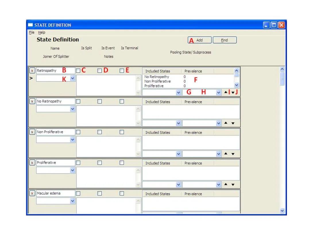
1. This form shows all states in the project. To add a new state, press the 'Add' button (A) on the top right of the form, and a new blank row will appear.
2. Enter the title of the state in the 'Name' box (B).
3. To define a state of type:Normal State: continue to next step.
   Event State: check box 'Is Event' (D).
   Splitter State: check box 'Is Split' (C).
   Joiner State: in drop-down box 'Joiner of Splitter' (K), select the name of the Splitter to be joined.
   Terminal State: check box 'Is Terminal' (E).
    
4. If the state is a process/pooling state, meaning that it contains other states, make sure all the "child states" within the process have been created first (repeat from step 2). Next, select a "child state" from the drop-down box (G), and click the up arrow button (I). Repeat for all nested states. Remember, when a child state is a sub-process, all of its children are automatically included.
5. It is important to note that the order in which the child states of a sub-process are defined determine the sort order by which transitions are displayed to the user. So they should be defined sequentially. Note that once a sub-process has been referenced, it is difficult to make changes in the system since changes in a referenced sub-processes will be blocked by the system.
   Pooling states are defined for studies that their states combine more than one model state together. The user should define the prevalence of these states. Using the software, pooling states are defined similar to sub-processes with a nonzero prevalence value defined in box (H) before pressing the button (I).
    
6. When finished, close the States form to save the states. This will trigger validity checking of the data entered; if no error message is displayed, then the data has been saved to memory. Note that the information is not yet saved to a file.

8.3 Removing States from a Process

To remove a state from a process:

1. In the States form, identify the process that you wish to modify.
2. Highlight the state you wish to remove in the Included States box (F) of that process.
3. Click the down arrow (J) to remove the state. Note: the state will not be completely deleted, it will only be deleted from the process.

To permanently delete a state:

1. Remove the state from any processes, using steps above. If the state is itself a process, delete all reference to it from studies that use it as a main process. This may require deletion of other entities and may be difficult if the deletion candidate was extensively used.
2. In the States form, identify the state that you wish to delete, and click the 'X' (delete) button at the left of that row. This may require deletion of other entities and may be difficult if the deletion candidate was extensively used.

8.4 State Indicator Parameters

Each State or Process has several state indicators associated with it. These state indicators are parameters that are set/reset during a simulation. All state indicators start with the name of the state where spaces are replaced by underscore characters '_'. The type of the state indicator is defined by the suffix at the end of the state name:

• Actual State Indicator - Contains no suffix to the state name. This state indicator will be set to 1 during simulation if the subject is present at this state at this simulation step.
• Entered State Indicator - Contains the suffix _Entered to the state name. This state indicator will be set to 1 during simulation if the subject is entered into this state at this simulation step. This state indicator is set to 1 only if the state was entered in this simulation step and will be reset if the individual stays in this state or leaves it.
• Diagnosed State Indicator - Contains the suffix _Diagnosed to the state name. This is a user controlled state indicator that is intended to indicate that a certain disease state has been diagnosed. The user is responsible for setting and resetting this state indicator. Note that at the start of simulation the Diagnosed state is considered to be the actual state.
• Treated State Indicator - Contains the suffix _Treated to the state name. This is a user controlled state indicator that is intended to indicate that a certain disease state has been treated. The user is responsible for setting and resetting this state indicator.
• Complied State Indicator - Contains the suffix _Complied to the state name. This is a user controlled state indicator that is intended to indicate that a subject has complied with a treatment. The user is responsible for setting and resetting this state indicator.

Sub-Process state indicators will be set to 1 if the user is in any state / sub-process within this sub-process. This means, for example, that the state indicator of the main process of a model used is simulation is always set to 1. States will generally behave the same with the exception of a simulation step where several sub-processes are joined by a joiner state. In this case, the sub-process indicators will be reset, while the state indicators will remain set until the next simulation step. This behavior allows cost calculations in this simulation step according to the states before the collapsing joiner state was reached.

9. Study/Model

9.1 Definitions of a Study and of a Model

Study: A study describes the data on the progression from one state to another state. This information is available in the literature and typically presented as incident counts from a given initial population count that reaches a specific state by the end of the study duration. Alternatively, study results can be reported in functional form.

Model: A specification of the disease progression created by the user within the system. The progression is defined as a set of states and processes, along with the transitions between these states. Transitions hold transition probabilities that describe transitions from one state to another.

Since both studies and models describe a disease process, they are bundled together in this system. The system distinguishes between study and model using the Study Length field. A model has a duration of 0, while a study has a duration greater than 0.

Studies often contain data regarding part of the disease model being studied, and are generally simpler in structure than models. Actually, they are restricted to a single sub-process. Studies are related to estimation projects, where they are used to provide information to estimate unknown model parameters. These parameters can then be calculated during an estimation process. Models with known transition probabilities can be used in simulation projects.

9.2 Working with Studies/Models

9.2.1 Creating a Study/Model

From the main window, click the 'Study/Model' on the left navigation pane.

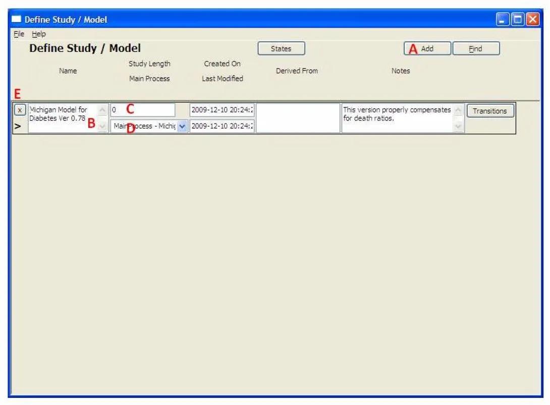
1. This form shows all of the studies and models in the project. To add a new study or model, press the 'Add' button (A), and a new row will appear in the table.
2. Give the study/model a name (B).
3. Set the Study Length (C). NOTE: as stated above, a model has a length of 0, and a Study has a length of greater than 0.
4. Select the Main Process from the drop-down (D). For a Study, The main process can contain only normal states, event states and pooling states. No sub-processes are allowed. The main process of a model can be much more elaborate and contain nested sub-processes. Double clicking on the field will open the states form and allow creation of the requested sub-process. Note that upon return the last state created will appear in the drop box.
5. Click on the Transitions button to define transitions related to the Study/Model. Note that transitions of a study will hold existing information whereas transitions of a model will hold probabilities.

6. Close the form or move to the next record to save the entry. This will trigger validity checking of the data entered and if no error message is displayed, then the data has been saved to memory. Note that the information is not yet saved to a file.

   9.2.2 Removing a Study/Model

   Open the Study/Model form. Identify the row to be removed, and click the 'X' (delete) button for that row. This may require deletion of other entities and may be difficult if the deletion candidate was extensively used.

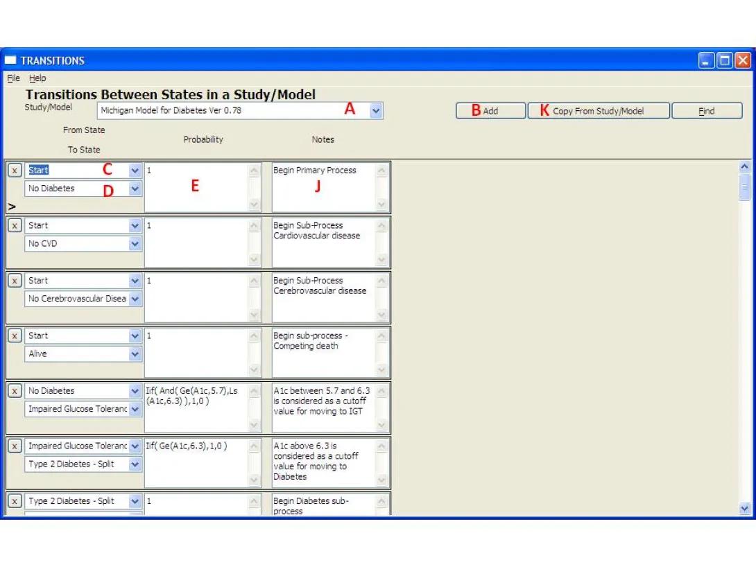
1. This form shows the transitions for a given Study/Model. Select the Model to be used from the drop-down box (A). Note: if the Transitions page was opened from the Study/Model page, that Study/Model will be selected and the combo box will be grayed out.
2. Click the 'Add' button (B).
3. Select the origin state for the transition (D).
4. Select the destination state for the transition (E).
5. Enter the transition probability in the box (F) as an expression, which may or may not include a Parameter. Parameters can be directly selected as the expression using the drop-down list.
6. Close the form to save the entry.

10.1.2 Removing Transitions

Identify the row that will be removed, and click the 'X' button (C) in that row. This may require deletion of other entities and may be difficult if the deletion candidate was extensively used.

10.2 Transitions for Studies

Defining study transitions is related to parameter Estimation. Study transitions may mean different things depending on the cases described below.

10.2.1 Creating Transitions for Studies

1. From the main window, click 'Transitions' on the left navigation pane.

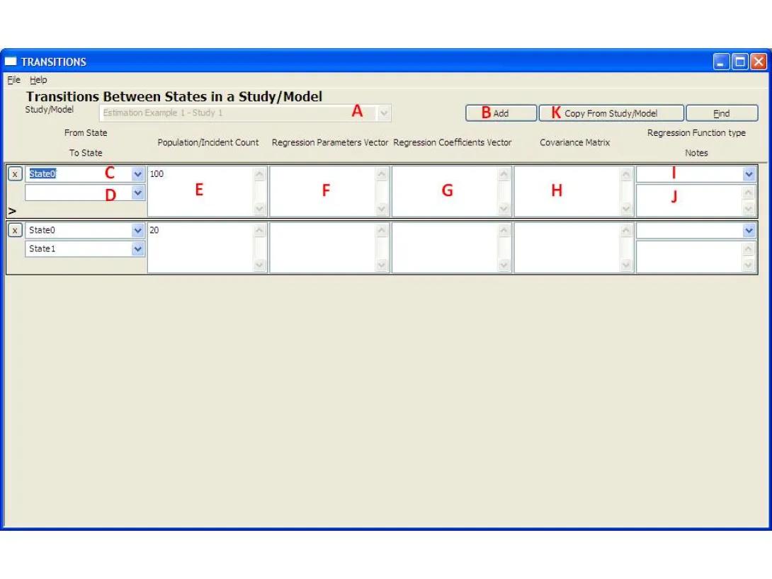
1. This form shows the transitions for a given Study/Model. Select the Study to be used from the drop-down box (A). Note: if the Transitions page was opened from the Study/Model page, that Study/Model will be selected and the combo box will be grayed out.
2. Click the 'Add' button (B).
3. Select the origin state for the transition (C).
4. Select the destination state for the transition (D). Leave blank to indicate initial population count of the study.
5. (Optional) Enter the Initial Population Count / Incident Count in the box (E). This field should be left blank for regression studies and filled for studies that report incident counts. Note that studies will in many cases require two transitions, the first for indicating initial count of people starting at a certain state, and the second for indicating the number of people ending at the end state at the end of the study. Both transitions will start at the same state, the first will have no end state indicating initial population count and the latter will define the ending state indicating the incident count reaching this end state.
6. (Optional) Enter a 'Regression Parameters Vector' (F). This field should be left blank for studies that provide results as incident counts. For a regression study it must be filled with a vector of the form [param0, param1, ...] that contains the reported regression parameters. If a bias term is reported, it is represented as the value 1 rather than a parameter name. This vector is multiplied by the Regression Coefficient Vector when creating the regression equation reported in the study.
7. (Optional) Enter a 'Regression Coefficients Vector' (H). This field should be left blank for studies that provide results as incident counts. For a regression study it must be filled with a vector of the form [coef0, coef1, ...] that contains the reported regression coefficients associated with the Regression Parameters Vector. Note that both vectors should be of the same size. This vector is multiplied with the Regression Parameters Vector when creating the regression equation reported in the study.
8. (Optional) Enter a 'Covariance Matrix' (I) or select one defined as a parameter from the drop-down list. This field should be left blank for studies that provide results as incident counts. For a regression study it must be filled with a matrix that contains the reported covariance matrix associated with the Regression Parameters Vector. Note that the Matrix should be of a size compatible with both vectors.
9. Close the form or move to the next record to save the entry. This will trigger validity checking of the data entered and if no error message is displayed, then the data has been saved to memory. Note that the information is not yet saved to a file.

10.2.2 Removing Transitions

Identify the row that will be removed, and click the 'X' button (C) in that row. This may require deletion of other entities and may be difficult if the deletion candidate was extensively used.

10.2.3 Copying Transitions from Another Study/Model

It may be desirable to build or modify a model/study by copying transition information from another model/study. The systems support this sort of copy using the following steps:

1. Initiate the transitions copy by pressing the Copy From Study/Model button (K). The following form will appear:

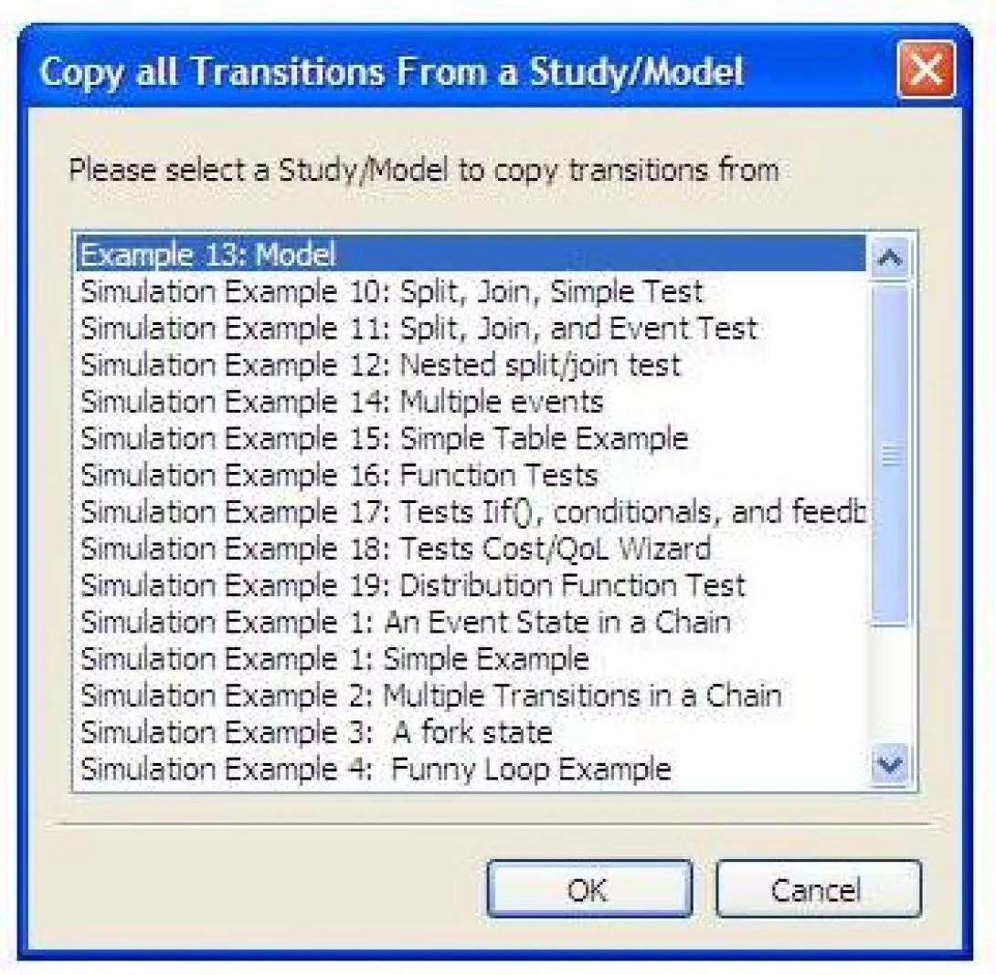
1. Select Study/Model you wish to copy the transitions from by clicking on it.
2. Press OK to initiate the copy or Cancel to abort the copy operation.
3. If the operation was not aborted, the system will bring a message indicating how many transitions were successfully copied. Dismiss this dialog box by pressing OK and the transitions form will display the copied transitions.

Note that this operation is useful while creating variations of a specific model that change the state/sub-process hierarchy. The copy transitions operation will try to copy all the transitions from the source model to the destination model. However, some transitions may not be copied as these may violate validation rules. Here are examples of transitions that will not be copied:

• Transitions that are already defined by states in the destination model will not be copied from the source model.
• Transitions where at least one of the states does not exist in the destination study/model will not be copied.
• Transitions that will violate the sub-process hierarchy will not be copied. For example if the to/from states are not in the same sub-process in the destination model.

11. Populations

A population (also referred to as population set or data set) represents a pool of subjects and their characteristics. A populations can be either input as data (to be used in a Simulation or an Estimation), or by specifying a distribution (to be used in Estimation or for randomly generating population sets).

11.1 Creating Populations

From the main form, click the 'Populations' button on the left-hand navigation pane. Note that this form can also be accessed by drilling down from the project form.

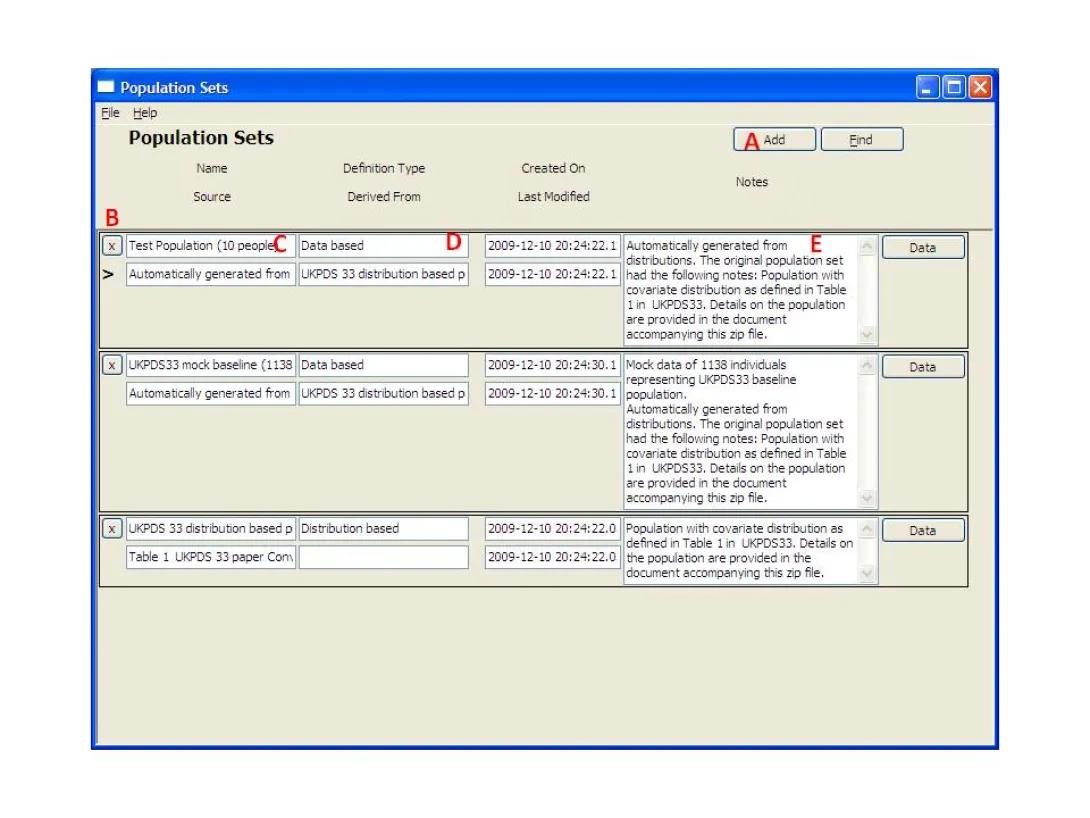
1. This form shows the population groups. Click the 'Add' button (A), and a new row will appear.
2. Enter the name for the population set in the box (C).
3. Click the 'Data' button (E) to define the population characteristics and associated data/distributions. The following form will appear.

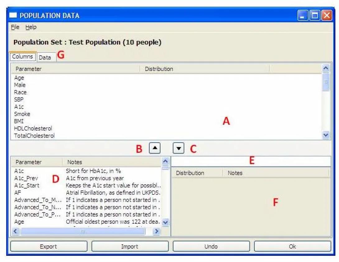
1. To input a population as data: Add a characteristic by selecting a parameter from the table in the lower left (D) and Click the up arrow (C). To remove a row, highlight it, then click the down arrow (B). After all the population characteristics have been added, press the Data Tab and fill in data for the chosen parameters for each individual. The data can also be imported from a file using the Import button. To view or change the data, press the data tab (G).
2. To specify a population by its distribution: Add a characteristic by selecting a parameter from the table in the lower left (D). Additionally, define the distribution expression in the text box (E), or select a distribution from the table in the lower right (F) and it will appear in (E). Click the up arrow (B) to add a row that combines the distribution and the parameter. To remove a row, highlight it, then click the down arrow (C).

NOTE: When attempting to duplicate a population defined by characteristics published in the literature, it is essential to recognize that the characteristics are not independent. For example, systolic and diastolic blood pressure are very highly correlated (r = ~0.8) and height and weight are also correlated (r ~ 0.5). For example, if height and weight are generated independently, it is likely that some subjects will have extreme body mass indices (BMIs) (i.e., a low weight in a very tall person may yield a physiologically unrealistic low BMI and conversely). Correlated covariates can be generated within the system, by first generating one covariate and then making the second covariate depend on the result of the first (i.e., express the second covariate by a regression function that is dependent on the first covariate).

11.2 Removing an Entire Population

Identify the population, and click the 'X' (delete) button. This may require deletion of other entities and may be difficult if the deletion candidate was extensively used.

11.3 Generating new population data based on distributions

The system supports the automatic generation of a population set defined by distributions of its characteristics. This feature can be used to automatically generate population sets in the system according to distributions provided in the literature. To perform these tasks, the following steps should be taken:

1. Follow the steps defined above in Creating Populations to define a population set defined by distributions that were defined in the previous step.
2. Select the desired distribution based population. The population set should read "Distribution based" in the Definition Type field (D).
3. Right click the mouse and a pop up menu will appear. Select the entry "Regenerate New Population Data from a Distribution".
4. A new input dialog window will appear and will ask for the population size to be generated. Enter the desired number and press OK.
5. The system will generate a new population set filled with data that was generated according to the distributions defined in the originally selected distribution population set. The system will place this population set at the end of the list and will focus on it so the user can modify it.

Note that generation of a data based population from distributions is controlled by multiple system option parameters that are listed in Parameters.

12. Parameters

Parameters are used for various purposes by the system. Parameters can specify covariates that will change during simulation or define a demographic characteristic of a subject. They can define constants and other values that can be reused during simulation. They also can be defined by a user-specified function and then used in subsequent functions as a symbol/shorthand for the user specified function; i.e., they may replace complex mathematical expressions or random generators in multiple functions.

Parameters are classified according to Parameter Types and may have different Parameter Validation Rules and data stored within them as explained below.

12.1 Parameter Types

The following parameter types can be defined by the system.

• Covariate - Specifies a covariate, a variable or a function of variables, that describe a subject; it can be referenced by many entities in the system. Examples of covariates are: Age, Gender, and Blood Pressure. A covariate can also be defined in functional form and contain an expression that references other covariates such as BMI_Over_30 = Max(BMI-30,0). See parameters of type Function below for further information. When specified as a functional form, the parameter is equivalent to a user defined function and, whenever used, it will be replaced by the expression it holds. Note that if this function includes a random number generator, a different value of the generator will be used each time the function is invoked. The default validation rule for this type of parameter is Number.
• Intervention - Reports whether or not the intervention occurs. It names a column in a result table where information will be stored about whether the intervention occurred. For example, if an ACE inhibitor was administered, the value of ACE_inhibitor will be set to one; otherwise, it is zero. Default validation rule for this type of parameter is Integer [0,1].
• Cost - Provides information on costs associated with a specific state. For example the parameter YearlyCost may include all costs associated with it. Cost parameters hold scalar values. Costs are calculated either through a Cost Wizard expression or through a mathematical formula that uses other parameters. Default validation rule for this type of parameter is Number [0,Inf].
• Quality of Life - Provides information about quality of life associated with a specific state. It is the name for a column in a result table where information will be stored about the quality of life. This is similar to cost with a different scale. Quality of life can be calculated either through the Cost Wizard or through a mathematical formula that uses other parameters. Default validation rule for this type of parameter is Number [0,1].
• Probability - May be used to specify a transition or prevalence probability. This may be used in defining characteristics of a sample (i.e., the prevalence of a covariate) or to define a parameter that is used in the simulation. Default validation rule for this type of parameter is Number [0,1].
• Transitions - the probability to move from one state to another; e.g., the probability of transition from Normal CVD to Angina. Default validation rule for this type of parameter is Number [0,1].
• Coefficient - These parameters are used as multipliers of covariates/evaluation/treatment parameters within transition formulas. These can either be determined during the estimation phase or assigned manually in phase 0 of simulation. Default validation rule for this type of parameter is Number.
• Function - gives a name for a function that can be used later during calculations. Each time the function name is used, it will be replaced by the expression that it represents. For example, a function that increases age may be called AgeIncrease and hold the function Age+1. When a function parameter is encountered in an expression, it is replaced by its contents during evaluation. This way the user can specify a user defined function that whenever used, will be replaced with the expression it holds. Note that if this function includes a random number generator, a different value of the generator will be used each time the function is invoked. Consider for example a parameter called CappedGaussian that generates random numbers using a Gaussian distribution with mean=0 and STD =1 that is restricted to the range from -3 to +3. This can be done by the user using the formula Min(Max(Gaussian(0,1),-3),3) to define this function type parameter. After definition in the parameter form, CappedGaussian can be used in any expression in the system during simulation or population generation from distributions. Whenever this parameter is encountered during simulation, a new random number will be generated on the fly; that is, reusing CappedGaussian will generate a new random number rather than return the same value. This is different than most other parameter types that generally hold values that are assigned to them. Default validation rule for this type of parameter is Expression.
• Table - A table parameter will hold both the definition of the table and the values of the table. The table will be defined by a unique name just like any other parameter. For example Table1. The table can hold multidimensional data along with dimension names, dimension ranges and table cell values. When the name of the table is used in an expression, the system will return the entry in the table corresponding to the subject's current values for the dimension names. Default validation rule for this type of parameter is Table.
• Vector/Matrix - Vectors and Matrices can hold arrays of numbers or parameters representing numbers. Vectors are one dimensional and matrices are two dimensional. Their representations are very similar. Default validation rule for this type of parameter is Matrix.
• Constant - Similar to a function, but constant. It is a general way to store constants and assign them a name. Default validation rule for this type of parameter is Number.
• State Indicators - These cannot be changed by the user, but can be used in expressions and other system functions. Parameters represent states in the system. For each state created in the system, there will be five parameters with a similar name and a different postfix. The name of the parameters will be the same as the state where non alphanumeric characters will be replaced with underscore characters and a postfix of 'Diagnosed' or 'Treated' or 'Complied' or 'Entered' will be assigned. For example for the state 'Survive MI' there will be 5 state indicator parameters called Survive_MI, Survive_MI_Diagnosed, Survive_MI_Treated, Survive_MI_Complied and Survive_MI_Entered . These parameters can be used in an expression during simulation and will represent the actual, diagnosed, treated, and entered states respectively. The value in the parameter associated with the state will be set to one if an individual is in this state in a simulation. It will be zero otherwise. For example, if for the state 'Survive MI' the value of the parameters can be Survive_MI=1, Survive_MI_Entered=1, Survive_MI_Diagnosed=0, and Survive_MI_Treated=0 Survive_MI_Complied=0 meaning that the individual is in actual state 'Survive MI' and has just entered it, while this is not the diagnosed or the treated state. For pooled states that represent sub-processes, this will mean that the state indicator parameter values will be set to 1 if the state associated with the sub-process and the individual will be set to 1. For example, if 'CVD' is representing a sub-process containing 'Survive MI'. Then the values of the state indicators can be Survive_MI=1, Survive_MI_Entered=1, meaning as before that the individual actually entered the state of MI_Survive and therefore CVD=1. If CVD=0 this means that it has not been entered and therefore Survive_MI=0. The validation rule for this type of parameter is Integer [0,1].
• Distribution - Provides information on the distribution of characteristics of a population. It is similar to a function and provides the capability of defining a marginal distribution for a covariate or intervention parameter. Note that the form of the function used as a distribution parameter will be similar to that of a random generator function. Constants are allowed, yet general expressions that are not distributions are blocked. Default validation rule for this type of parameter is Distribution.
• System Reserved - The parameter table in the Database may be used by the system to store temporary parameters to help in calculations and may contain reserved names that cannot be used by other parameters. For example Time can be reserved by the system. Also, internal functions names would be in the system reserved list so that a user will not use these by mistake. It is not allowed to change System Reserved parameters.
• System Arrays - May be used to define an initial set of default initial guesses for all parameters for an estimation project. Default validation rule for this type of parameter is Matrix.
• System Options - These names are set by the system by default; their values can be modified by the user to change functionality of the system. Default validation rule for this type of parameter is Number. Here is a short description of these parameters by categories of influence:

  • System Option Parameters Affecting Simulation and Population Generation from Distributions

    • ValidateDataInRuntime: A number that defines the level of validity checking of expressions during simulation and population generation from distributions. The following levels are supported:
      • 0: No validity checking.
      • 1 or greater: Check that probabilities are within 0 and 1 and check that these sum to 1 when leaving event states and joiner states, and check that a value assigned to a parameter fits the validation rules defined for it.
      • 2 or greater: Check that function parameter validity rules are honored during calculation of expressions - this is the default option.
      • 3 or greater: Impose extra redundant validation checks on all phases of calculation.
    • NumberOfErrorsConsideredAsWarningsForSimulation: The number of times the system will accept parameter validity violation errors during simulation as warnings and will not stop simulation. When this number of errors is reached, the system will raise a fatal error to the user and stop simulation. The error messages can be seen on the console window.
    • NumberOfTriesToRecalculateSimulationStep: The number of times that the system will force recalculation of the same time step if an error was raised during this time step. If unsuccessful after this number of recalculations then force recalculation of the entire individual from the first time step.
    • NumberOfTriesToRecalculateSimulationOfIndividualFromStart: The number of times an individual will be recalculated from start in case errors appeared during simulation that forced restarting calculations. If this number of tries is reached, a fatal error is raised that stops simulation.
    • SystemPrecisionForProbabilityBoundCheck: This is a very small tolerance number that defines how accurate will be fatal error checks for probabilities if ValidateDataInRuntime>=1. This number allows overlooking machine precision issues.
    • RepairPopulation: This integer defines the level the system will try to correct a population set to fit a model before simulation. The following levels are supported:
      • 0: No repairs are made and errors are generated. This forces the user to match population set parameters and model parameters very carefully, including process names.
      • 1 or Greater: The system will attempt to figure out values for process state indicators and other states in the process according to the model structure and according to state indicator values defined in the population set.
      • 10 or Greater: The system will remove individuals with empty values in the population data before simulation, and therefore avoid generating an error that will stop the simulation process.

    • VerboseLevel: Defines how much information to output during simulation.

      Here are supported levels for output from population generation from distributions:

      • 3 or greater: Record random seed number on file that will be created at the start of population generation from distributions.
      • 7 or greater: Record generated population set on file. This would be a pickled python list object.

      • 10 or greater: Print an announcement each time a new individual starts generation. Also print a generation summary at the end of of population generation from distributions.

        Here are supported levels for output from bridging population set and model definitions before simulation:

        • 1 or greater: Print summary of the bridge process.
        • 5 or greater: Print a message if deleting a record due to a missing value.
        • 10 or greater: Show each process set by the system due to a child state.

        Here are supported levels for output from simulation:

        • 3 or greater: Record random seed number on file that will be created at the start of simulation.
        • 7 or greater: Record simulation results set on file.
        • 10 or greater: Print an announcement each time a new individual starts simulation. Also print a simulation summary at the end of simulation.
        • 20 or greater: Print an announcement each time an individual starts a new repetition during simulation. Also print a message if recalculation of a repetition was forced due to error.
        • 30 or greater: Print an announcement each time step during simulation. Also print a message if recalculation of a time step was forced due to error.
        • 40 or greater: Print an announcement for each state in the State Processing Queue (SPQ). This is highly advanced and requires deep understanding of the system.
    • RandomSeed: Defines a random seed to start both population generation and simulation. NaN is used to indicate that system time will be used as a random seed - essentially making numbers different each simulation.
    • NumberOfErrorsConsideredAsWarningsForPopulationGeneration: The number of times the system will accept boundary violation errors as warnings and will not stop during population generation from distributions. When this number or errors is reached, the system will raise a fatal error to the user. Error messages can be found on the console window.
    • NumberOfTriesToRecalculateIndividualDuringPopulationGeneration: The number of time the system will try to recalculate the same individual if a non fatal error is encountered during calculation of that individual. Once this number is reached a fatal error will be raised and generation of data from distributions will stop.

    System Option Parameters Affecting Estimation

    • Opt_SymbolicToNumericTolerance: A small number used by the system as a threshold to test the result before and after optimization by comparing symbolic calculation to numeric calculation.
    • Opt_UseMultiPhaseOptmization: A number from 1 to 3 signifying the number of optimization phases to use. Phases allow using different optimization parameters to reach the best optimization result.
    • Opt_GradientPerturbationH: A small number used as an interval during numerical derivation when calculating likelihood of optimization studies.
    • Opt_SkipDerivativesForLongExpressions: The length of the largest expression for which the system will calculate derivatives and use them during optimization. This calculation will be skipped for longer expressions.
    • Opt_LongExpressionsPrintSize: The maximum number of characters to print from an expression. If an expression print is cut, this will be noted to the user by a symbol.
    • Opt_SkipDerivativesIfMemoryError: Unless this variable is set to zero, the system will ignore memory errors generated if long expressions are derived and create expressions so long that may not fit in memory
    • OptPhase1_fmin_l_bfgs_b_approx_grad, OptPhase2_fmin_l_bfgs_b_approx_grad, OptPhase3_fmin_l_bfgs_b_approx_grad: The parameter approx_grad to be passed to the optimization routine during optimization phases 1,2,3 respectively. For further details click here
    • OptPhase1_fmin_l_bfgs_b_m, OptPhase2_fmin_l_bfgs_b_m, OptPhase3_fmin_l_bfgs_b_m: The parameter m to be passed to the optimization routine during optimization phases 1,2,3 respectively. For further details click here
    • OptPhase1_fmin_l_bfgs_b_factr, OptPhase2_fmin_l_bfgs_b_factr, OptPhase3_fmin_l_bfgs_b_factr: The parameter factr to be passed to the optimization routine during optimization phases 1,2,3 respectively. For further details click here
    • OptPhase1_fmin_l_bfgs_b_pgtol, OptPhase2_fmin_l_bfgs_b_pgtol, OptPhase3_fmin_l_bfgs_b_pgtol: The parameter pgtol to be passed to the optimization routine during optimization phases 1,2,3 respectively. For further details click here
    • OptPhase1_fmin_l_bfgs_b_epsilon, OptPhase2_fmin_l_bfgs_b_epsilon, OptPhase3_fmin_l_bfgs_b_epsilon: The parameter epsilon to be passed to the optimization routine during optimization phases 1,2,3 respectively. For further details click here
    • OptPhase1_fmin_l_bfgs_b_iprint, OptPhase2_fmin_l_bfgs_b_iprint, OptPhase3_fmin_l_bfgs_b_iprint: The parameter iprint to be passed to the optimization routine during optimization phases 1,2,3 respectively. For further details click here
    • OptPhase1_fmin_l_bfgs_b_maxfun, OptPhase2_fmin_l_bfgs_b_maxfun, OptPhase3_fmin_l_bfgs_b_maxfun: The parameter maxfun to be passed to the optimization routine during optimization phases 1,2,3 respectively. For further details click here

12.2 Parameter Validation Rules

Parameters can be assigned validation rules to verify that the result of the formula is of the specified type. They do not modify the Parameter in any way. a Validation Rule can be:

• Number - accepts any floating point number such as 1.23345 or -0.123 or 1.2e3, subject to specified limits.
• Integer - accepts integers, such as 1,2,3.
• Expression - accepts system or user defined functions and parameters in general mathematical expressions such as Age+1, or Exp(-1.234), or Max(Age,20) +1. Parameters in a validation rule expression are different than other parameters that generally hold values after assigned to them. A parameter validated as an expression is actually a function that forces evaluation of a defined expression rather than hold a value. See Expressions for additional information.
• Matrix - checks the syntax of the matrix and allows only vectors of dimension 1 and matrices of dimension 2. Examples of vectors can be [1,2,3,4] or [1,Age,BP], whereas matrices will have the format [ [ 1,2,3], [ 4,5,6], [7,8,9] ] . Vectors and matrices are used during Estimation.
• Distribution - checks the syntax of the expression for a valid definition of the statistical distribution expressions. Distributions are used during Estimation. The expression will be limited to be a Distribution function name used in a function form to generate random numbers. See Expressions for additional information.
• Table - checks that the parameter holds a multi-dimensional table entity. This forces additional syntax checks limited to tables. See Expressions for additional information.

When defining a parameter with the validation rule Number, Integer, Expression, Table, the user can define additional validation rule parameters of the type [min, max] that will define bounds for this parameter. For example a user who wishes to define a Boolean parameter, should define an integer with the validation rule parameters of [0,1]. Another example is a user who wishes to define a positive integer should define a parameter of the type integer with the validation rule parameter of [0,Inf]. By default and unless specifically requested otherwise by the user by changing the appropriate system options, validation rules and validation rule parameters are checked during simulation at each step to verify values are within the allowed ranges.

Default validation rules and validation rule parameters are defined by the parameter type as stated above.

12.3 Working with Parameters

Creating Parameters

From the main form, click the 'Parameters' button on the left-hand navigation panel. The following form will appear:

To see all parameters, make sure 'ALL User Accessible' is selected, and press 'OK'. You can also decide to check only the parameter types of interest to view instead seeing all parameters. Then the parameter form will appear:

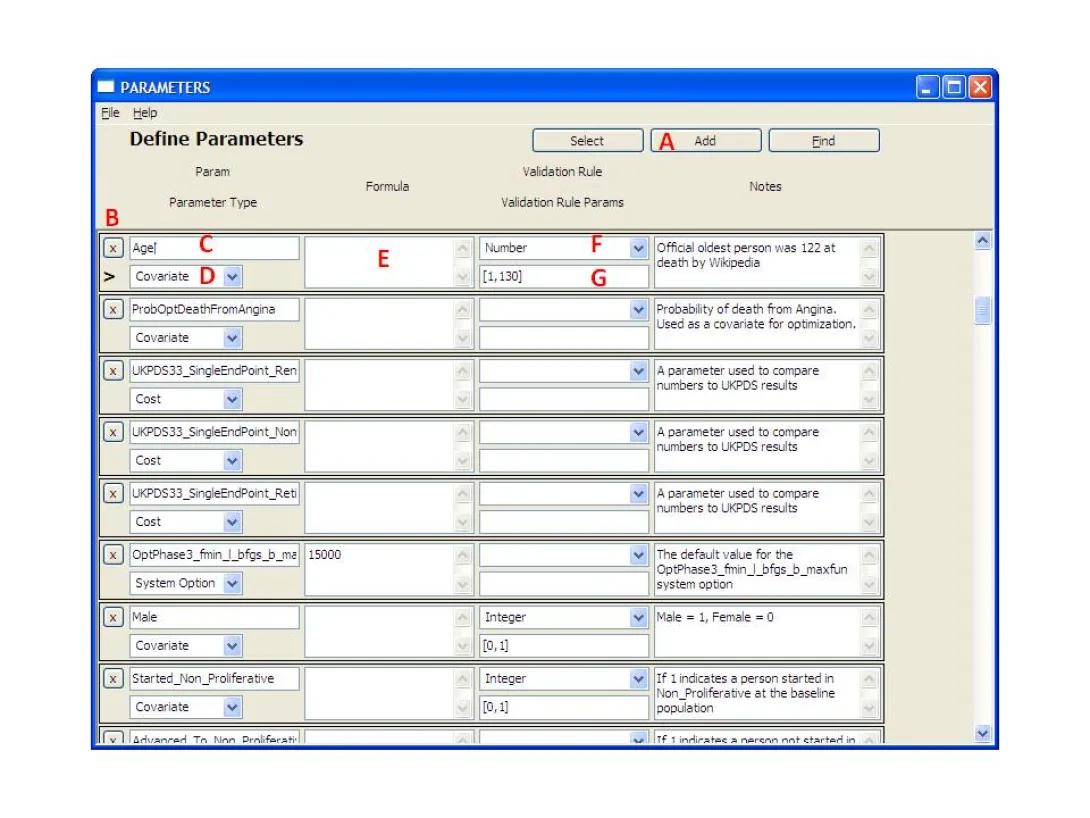
1. This form displays the Parameter details. To add a new Parameter, click the 'Add' button (A), and a blank row will appear.
2. Enter the Parameter name in the box (C).
3. Pick the Parameter Type from the drop-down (D).
4. Optionally enter a Formula in the box (E). When this entry is left empty, the user is responsible to assign a value to the parameter elsewhere in the system. An expression defined in the formula defines a substitution expression that will be calculated on the fly, whenever encountered, and may receive different values if it includes a random number generator. The formula is a general expression, yet it is restricted by the parameter type and validation rules.
5. Optionally Pick a Validation Rule from the drop-down (F), which will verify the output type of the Formula. If you do not pick a validation rule, it will be defined by default by the system according to the parameter type.
6. Optionally Enter the Validation Rule Parameters in the box (G). A Validation Rule will define the range of values the parameter may have within brackets. If you do not pick a validation rule, it will be defined by default by the system according to the parameter type.7
7. Close the form or move to the next record to save the entry. This will trigger validity checking of the data entered and if no error message is displayed, then the data has been saved to memory. Note that the information is not yet saved to a file.

Note: The parameters form can accessed from other forms by double clicking a field that requires a parameter. This allows creating parameters on the fly while working from another form.

13. Expressions

The system uses expressions in parameters and in simulation rules. Expressions include mathematical and logical formulas. Expressions can be a simple as 1+2; they can use another parameter as in Age +1; They can be complex expressions using mathematical functions as in Exp(-Age); They can even use if statements as in Iif(Gr(Age+1,50),1,0); These expressions can also represent tables as in Table(1,3,0,0.5,1,Age,NaN,20,30,40) . These formulas may contain, as literals parameter names (including parameters that hold values, parameters that specify user defined functions, state indicator names, and some reserved words), mathematical operators, system built in functions. Below is a list of allowed operators:

13.1 Supported arithmetic functions

• + : Addition operator
• - : negative/subtraction operator
• * : multiplication operator
• / : division operator (note that integers will be treated as floating point numbers)
• ** : power operator

13.2 Other supported literals

• () : Parenthesis to determine the order of the calculation
• [,] : brackets enclosing comma separated values describe vectors and matrices. Note that this type of expression is limited to defined vectors and matrices

13.3 A list of comparison operators

• Eq(x1,x2): will return 1 if x1=x2 and 0 otherwise
• Ne(x1,x2): will return 1 if x1<>x2 and 0 otherwise
• Gr(x1,x2): will return 1 if x1>x2 and 0 otherwise
• Ge(x1,x2): will return 1 if x1>=x2 and 0 otherwise
• Ls(x1,x2): will return 1 if x1<x2 and 0 otherwise
• Le(x1,x2): will return 1 if x1<=x2 and 0 otherwise

13.4 A list of Boolean operators

In the following Boolean operators, the results are either 1 or 0. Any argument that not zero is considered be true and zero is treated as false.

• Or(x1,x2,x3�): will perform a Boolean OR operation on two or more inputs
• And(x1,x2,x3�): will perform a Boolean AND operation on two or more inputs
• Not(x): will perform a Boolean Not operation on a single input
• IsTrue(x): will return 1 for a numeric x that is not 0. Will return 0 otherwise.

13.5 A list of special math related functions and symbols

Note that these may be platform dependent. Boolean operators treat NaN (Not a Number) as false as well as any other non-number type such as a vector/matrix.

• Inf, inf: will be recognized by the system as infinite. This symbol is not to be used in mathematical calculations as it may generate error. It can be used for bound checks for parameters.
• NaN, nan: will be recognized by the system as not a number. Note that comparison of NaN to any number including NaN will return False. Arithmetic operations using NaN produce NaN and may raise errors and therefore should be avoided.
• IsInvalidNumber(x): will return 1 for x=NaN or for a non numeric type such as a vector , 0 otherwise
• IsInfiniteNumber(x): will return 1 for x=-Inf or x=Inf, 0 otherwise
• IsFiniteNumber(x): will return 1 if x is a finite number, 0 if x is not a valid number or an Infinite number

13.6 Mathematical functions

• Exp(x): exponential
• Log(x,n): logarithm of base n
• Ln(x): natural logarithm
• Log10(x): decimal logarithm
• Pow(x,n): power operator similar to **
• Sqrt(x): square root operator similar to **0.5
• Pi(): the mathematical constant approximately equal to 3.14159

13.7 Other functions

• Mod (x,n): Modulus of base n
• Abs(x): Absolute value of x
• Floor(x): closest integer equal to or below x
• Ceil(x): closest integer equal to or above x
• Max(a1,a2,a3�): the maximum value in the list
• Min(b1,b2,b3�): the minimum value in the list

13.8 Statistical Distributions - Random number generators

Note the difference in number of arguments from the CDF shown in the next section. These random functions can be used to define the Distribution of parameters:

• Bernoulli(p)
• Binomial(n,p)
• Geometric(p)
• Uniform(a,b) : the arguments a and b define the lower and upper limits of the interval
• Gaussian(mean,std)

13.9 Statistical Distribution - CDF evaluation at point x

Note the difference in number of arguments from the random functions shown in the section above. The last argument x represents the value at which the CDF will be calculated. These functions cannot be used to define the Distribution of parameters:

• Bernoulli(p,x)
• Binomial(n,p,x)
• Geometric(p,x)
• Uniform(a,b,x)
• Gaussian(mean,std,x)

13.10 Control and Data Access

• Iif(Statement,TrueResult,FalseResult): Returns TrueResult if Statement is not 0, FalseResult if Statement is 0.
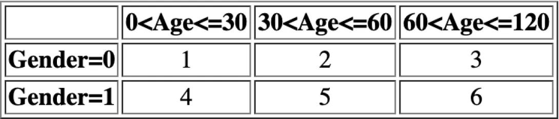
• Table (TableParameters): A multi-dimensional table. TableParameters are provided as a string of comma-separated values. The Table Input argument pattern is: D,N_1,N_2,...,N_D,V_1...V_(N1*N2*...*ND),M_1,R_1_0...R_1_(N_1)......M_D,R_D_0...R_D_(N_D). Where D defines the number of dimensions, N_i the dimension size for dimension i, V_i table values, M_i dimension names, R_i_j, the j range value definition item for dimension i . NaN value in R_i_0 means the dimension is discrete rather than continuous and the range bounds provided later represent values rather than lower and upper bounds associated with cells. For example Table(2,2,3,1,2,3,4,5,6, Gender, NaN,0,1, Age,0,30,60,120) defines a D=2 dimensional table with the dimensions M_1=Gender and M_2=Age. The levels of each dimension are defined by cutpoints which represent the lower and upper bounds for each interval; > lower bound and <= upper bound. When the dimension is categorical, such as Gender, the first cutpoint should be NaN, followed by the values of the categories. When the dimension is continuous, the first cutpoint is less than the minimum and the last cutpoint is >= the maximum. In our example, . the Gender Dimension has N_1 =2 categories with the discrete values of R_1_0 =NaN, R_1_1 = 0 and R_1_2 = 1, and the Age dimension has N_2=3 categories defined by R_2_0= 0<Age<=30= R_2_1, R_2_1= 30<Age<=60= R_2_2, R_2_2= 60<Age<=120= R_2_3.The values that the table holds are V1...V6=1,2,3,4,5,6. as can be seen in the following table:

13.11 Application specific

• CostWizard (FunctionType, InitialValue, CoefficientVector, ValuesVector): The function calculates costs or QoL according to FunctionType: If FunctionType=0, costs are calculated if FunctionType=1, Quality of life is calculated. Note that CoefficientVector and ValuesVector are vectors of the same size. The system returns an error if there is an incompatibility between parameters and coefficients or if the FunctionType is not 0 or 1. The cost/QoL function is calculated according to the formula presented in Zhou H, Isaman DJ, Messinger S, Brown MB, Klein R, Brandle M, Herman WH. A computer simulation model of diabetes progression, quality of life, and cost. Diabetes Care. 2005;28(12):2856-63. Note that the values associated with the cost/QoL can be changed by the user.

Note that missing values are not supported by the system. An exception is population data upload in which case missing data values are ignored by default in simulation.

14. Reports

The reports option provides users with the ability to view the information in textual form. Reports can include information about parameters, states, studies/models, transitions, population sets, projects, and results.

14.1 Generating a Report

Reports are generated in the context of the topmost open window. For example a report generated from the Study/Model window will generate a report describing a study/model and a report generated from the project window will describe the project.

To generate a report for a single entry in any form:

1. Select the row/record of interest.
2. From the menu bar at the top of the form, select File.
3. From the File menu select Single Report.

To generate a report regarding all the records in the form:

1. From the menu bar at the top of the form, select File.
2. From the File menu select Report All.

Either of these actions will open the Report Viewer form with the generated report:

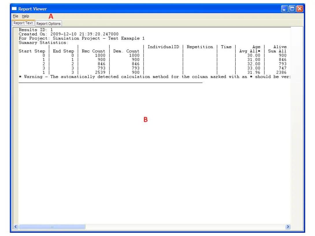
The user can view the report in the text area (B). Note that the reports are usually very wide and may not fit the screen and using the scroll bars to view the results may be necessary.

14.2 Saving the Report File

To save the report as text:

1. From the menu bar at the top of the Report viewer form, select File.
2. From the File menu select Save to save under a default file name. Select Save As to allow the user to modify filename/path.

Also note that portions of the report can be highlighted and copied into the clipboard to be pasted into other applications.

14.3 Changing Report Options

The report that first appears uses default options defined by the system. The context/formatting of most reports can be controlled by the user. Specifically the simulation results report is very extensive and has many options, whereas other reports use the Detail Level option.

To change report options, from the report viewer form select the Report Option tab (A). The following options form will replace the result tab:

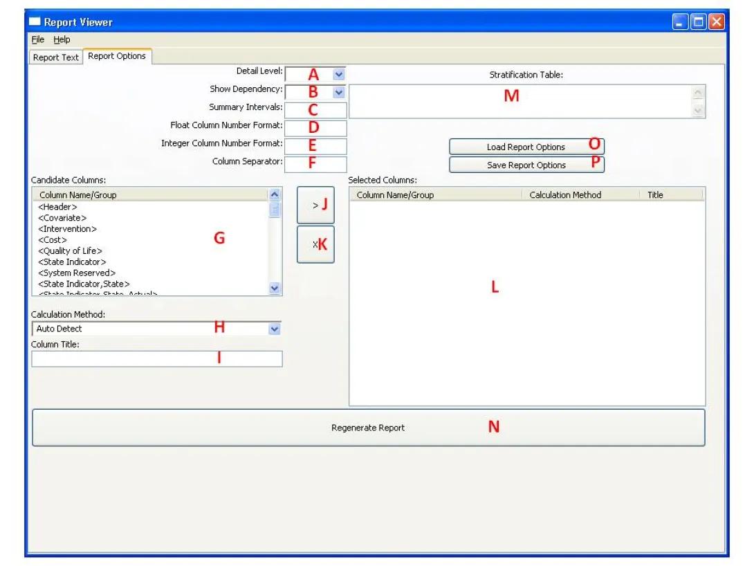
The user can now change report options using according to the following instructions:

1. Choose the appropriate Details Level from the drop box (A), or leave blank for a default of 0. This report option affects the reports for most entities. The higher the number the more details will be provided on the entity. In some cases, higher details level will drill down into other entities associated with the reported entity. Higher Detail Level will indicate more levels of drilling down.
2. Choose the appropriate Show Dependency from the drop box (B), or leave blank for a default of No. This report option affects the reports for most entities. If Yes is selected, the report will contain additional information regarding dependencies between entities, such as states and the associated state indicators etc. In addition, some expressions will be explained in a more readable fashion to the user.
3. Define an appropriate Summary Intervals (C) for a simulation results report, or leave blank for the default. This option defines a list of simulation step intervals for summary statistics in the report enclosed in brackets [a,b,c�]. Summary interval members can be defined as an integer such as 2 meaning a summary will be generated for every 2 simulation steps. Alternatively, a summary interval member can be specified by a nested set of [] in a [min,max] format such as [1,3] meaning the interval starts at simulation step 1 and ends at simulation step 3. The number 0 refers to the initial condition. Also if the number 0 is defined as a single member at the beginning of the list, this means simulation steps will be counted from the initial state rather from the first simulation step. Note the difference between 0 as a number compared to the range [0,0]. The first one means that counting time intervals starts at 0 instead or at the first simulation step, whereas the latter means to report the initial condition as a summary interval. Finally, the maximal interval of [0/1, Max] is always automatically included by the system at the end of the list. Where Max stands for the maximal number of simulation steps as defined in the project and 0/1 is dictated by the appearance of 0 in the list. If no specification is made, then the following default results are presented: each cycle, sequential five-cycle interval, sequential 10-cycle intervals and a summary of the entire range of cycles. To help understand these concepts, here are a few examples:
   • When there are two nonzero entries [a,b], then first each sequential 'a' cycles will be summarized followed by each sequential 'b' cycles. For example, the list [1,2] will mean generating summaries for every year starting at 1, i.e. equivalent to [1,1],[2,2],[3,3] etc. and then generating all summary intervals 2 years apart, i.e. equivalent to [1,2],[3,4],[4,6] etc. Finally the system will add the overall interval of [1, Max].
   • When an interval is embedded in a second set of [] such as [[a,b]], then the interval of cycle 'a' to 'b' will be summarized. For example, the list [[1,2]] will generate a single summary interval [1,2] and the system will add the overall interval of [1, Max].
   • When zero is specified, it modifies the summaries to start from cycle zero (the initial state. For example, the list [0,2] will generate the following summary intervals two years apart [0,1], [2,3],[4,5] etc. and then the system will add the overall interval of [0, Max].
   • The list [[0,2]] will generate a single summary interval [0,2] and the system will add the overall interval of [1, Max].
   • The number 1 alone will be recognized by the system as [1] meaning a summary interval for each simulation step i.e. [1,1] ,[2,2],[3,3] etc. and the system will add the overall interval of [1, Max].
4. Define appropriate Float Column Number Format (D) and Integer Column Number Format (E) for a report of the simulation results, or leave blank for the default. If one of these options is defined, the other one is required as well. These two options define how numbers will look at the summary section of the report. The format is based on the format available in the Python Language with the following modification. If the last character in the format string defining the float format is 'v' or 'V', this means relative precision with a desired precision compared to the max value of the column where the number of significant digits is specified before the 'v' or 'V'. Otherwise formatting is according to the string defined. Note that lower case 'v' means that each category of information, i.e. raw data or summary statistics, is dealt with separately when considering relative numbers. An upper case 'V' means that all numbers in the column are considered when determining the precision for that column. In simple words this option allows for displaying the precision in the context of all the numbers in the column. Note that this does not apply to integers. If these values are not defined the value is '%0.5v' for floats and '%i' for integers, where 0.5 means 5 nonzero digits and %i means the entire integer.
5. Define an appropriate Column Separator (F) for a simulation results report or leave blank for the default of '|'. This allows the user to define the character that separates columns. This is useful when importing the report text to a spreadsheet as this allows automatic separation of columns.
6. Define columns of interest to display in the simulation results report. This involves several operations as follows:
    
   1. Select a column/group from the candidate group list (G). Column names are parameters that exist in the result set and can be selected by name. This includes all state indicators of all types and all parameters defined in the initial population set and in the simulation rules. For ease of selecting entire groups of columns, these parameters are grouped by the system in several groups such as <Covariate> or <State Indicator>. A user can select a column or a group to allow flexibility. Note that the Group <Heading> has special treatment as it creates the header for the report.
   2. Select the calculation method to apply to the column from the drop box (H) or leave it as Auto Detect. In most cases the system will be able to deduce the desired calculation method from the list, which is the default. Yet the user can force a specific calculation method overriding the system auto detection mechanism. Possible calculation methods are:
      • Auto Detect: System automatically selects the calculation method from the list below according to the parameter characteristics and its use in the project. If this option is selected and there is ambiguity as to the calculation method required, the system will place an * in the report on this column and place a warning at the end of the report. A user should then verify that the calculation is proper and if needed manually select the calculation method for this column.
      • Func Over All Records - will apply Func to values from all the records in the summary interval. When Func=Sum, the system will sum the column values for all the records in the summary interval. It is useful to count the number of occurrences of a state in a population in a given summary interval. This is the default option for Booleans that are not demographics, e.g. State indicators. When Func=Average, the system will average the column values for all the records in the summary interval. It is useful to find the average value of a covariate changing during simulation in a given summary interval. It is equivalent to dividing the sum over all records by the total number of all records in the interval. This is the default option for non-Booleans that are not demographics, i.e. may be affected during the simulation. When Func = STD, sample standard deviation is calculated using the method of provisional means. When Func = Min or when Func = Max then the minimal or maximal value of all records in the interval is reported. Func = Valid Count will return the non NaN count.
      • Func Over Demographics - will apply Func to values in records entering the summary interval. When Func=Sum, the system will sum the column values for the first year in the summary interval. Demographic characteristics are considered as the value defined in the first year in the interval. Demographics values should not change during simulation steps. This option can be used to represent the number of occurrences of a state in a population entering the summary interval. This is the default option for Booleans that are unaffected by the simulation i.e. non state indicators not in the affected list of the simulation project. When Func = Average, the system will average the column values for the first year in the summary interval. Demographic characteristics are considered as the value defined in the first year in the interval. Demographic values should not change during simulation steps. This option can be used to represent the average of a covariate in a population entering the summary interval. It is equivalent to dividing the sum over demographics by the total number of records entering the interval. This is the default option for non-Boolean parameters that are in the affected list of the simulation. When Func = STD, sample standard deviation is calculated using the method of provisional means. When Func = Min or when Func = Max then the minimal/maximal value of demographics records entering the interval is reported. Func = Valid Count will return the non NaN count.
      • Func Over Last Observations Carried Forward - will apply Func to the last record of each individual. The max time record, i.e. either the record in the year of termination, or the last year record, is considered. Note that every individual will have exactly one record for each repetition. Func can be Sum, Average, STD, Min, Max, Valid Count.
      • Record Count - This calculation option will count the number of records within the summary interval. It is useful to show the denominator used for Average Over All Records defined above, in case it is of interest to the user.
      • Demographic count - This calculation option will count the number of records within the first year of a summary interval. In other words it will return the number of individuals entering the summary interval. It is useful to show the denominator used for Average Over Demographics defined above, in case it is of interest to the user.
      • Interval Start: This option will return the simulation step number defining the summary interval start. This option ignores the column numbers and will work with any column the same. Note that this is used by the system in the <Header> column group and in most cases will not be needed for the user again.
      • Interval End: Similar to Interval Start above with the difference that it returns the last simulation step number in the summary interval.
      • Interval Length: Similar to Interval Start above with the difference that it returns the number of simulation steps represented in the summary interval such that Interval Length = Interval End - Interval Start +1
      • No Summary - No summary is returned for the column. It can be used to create spaces in a report.
   3. Optionally select an alternative label for the column name (I) or leave blank. By Default blank means that the column name will not change in the report.
   4. Add the column/group, calculation method, and label to the selected columns list (L) by pressing the button (J). The column will be added before the column selected in the selected column list (L), if none were selected, it will be added at the end. Pressing the x button (K) will remove a selected column from the selected columns list (L). Note that the order that appears in the selected columns list (L) will allow users to control the order the columns appear in the report as well as their calculation methods. Note that the same column may appear several times with different calculation methods associated to it. Note that by default the selected column list is blank, meaning all columns defined in the simulation with automatic calculation, with a default header group at the start of the report.
   5. Field (M) provides rules for stratification of simulation results. If left empty, results will be reported without stratification. If this field contains a valid table expression, the results will be presented stratified by the dimensions and the ranges that describe the table cells. The value of the table cells must be one of the following:
       
      0. No stratification
      1. Stratification by population demographics
      2. Stratification by entry demographics to time interval
      3. Stratification by record
7. When all options have been defined by the user, press on the Generate Report button (N) to regenerate the report. The system will then automatically bring back the Report Text tab with the new report. Note that for some cases, the regeneration of the report may take some time.

15. Utilities

With the details you already have, you should be able to conduct complicated simulation scenarios with various models and population sets. You are also able to produce reports to help analyze the simulations. Yet sometimes there is a need to get beyond the results of a single simulation, or there is a need to take the data outside the GUI. To support such manipulation, the system offers some python utilities that arrive with the system. The following text will explore these utilities and their usefulness by subject.

The utilities are python scripts that allow the user to perform special advanced tasks. Here is a brief list of these scripts:

• ConvertDataToCode.py : A utility that converts zip file generated by the system to a python script.
• MultiRunSimulation.py : A utility that allows running the same simulation multiple times outside the GUI. Useful for parallel processing on multiple computers. It can be used well with MultiRunSimulationStatisticsAsCSV.py to generate a summary statistics for repetitions.
• MultiRunCombinedReport.py : A utility that allows combining results from several runs of the same model and population set into a single report. The use of this utility allows running multiple simulations in parallel and combining their results.
• MultiRunSimulationStatisticsAsCSV.py : A utility that generates CSV summary reports from several runs of the same project. Combines well with MultiRunSimulation.py that generates input files for this CSV report. The output consists of mean,STD,median,min,max of report columns with regard to different simulation results.
• MultiRunExportResultsAsCSV.py : A utility that generates a CSV file containing the data from a set of result files.
• AssembleReportCSV.py : A utility that assembles a CSV file from multiple CSV files generated by MultiRunExportResultsAsCSV.py
• CreatePlotsFromCSV.py : A utility that constructs plots in a PDF file. The plot data is collected from a CSV file assembled by AssembleReportCSV.py
• CodeFromDocAndSpreadsheet.py : A python script that converts rule text from a word document and CSV file from a spreadsheet with populations into code and a model file. This script was created to handle a specific format used with the Michigan model documentation. This file relies on a very specific format of documents and remains undocumented and should be treated as an example for programmers that want to extend the system.

15.1 Invoking Utility Scripts

All these scripts are invoked using a similar manner. Therefore for explanation purposes we will refer to the script name, including the .py extension as: PythonScript.py. Whenever the name PythonScript.py is encountered, it should be replaced with the script name of interest.

The above scripts all start from the command prompt / terminal window. In Linux you can open a terminal window. In windows you can select the command prompt under the program group called accessories when you click on the windows start button on the lower left corner. On the windows start menu, you can also select run and then type cmd and then press Enter to launch the command prompt.

Once you opened the terminal, you will have to change directory to your working directory by typing:

cd WorkingDirectoryFullPath

Recall that your working directory is the directory you installed IEST and WorkingDirectoryFullPath means the full path name. To write the full directory name you can use the tab completion feature, or use drag and drop of a file into the command prompt window in windows and make corrections to the name that appears. Note that the directory separator on PC is the backslash character \ while on Linux it is a slash character / .

Once you are in the correct directory, you can invoke the script PythonScript.py by typing:

On Linux:

python PythonScript.py

On Windows:

c:\Python27\python PythonScript.py

Note that if you defined the python installation directory to be in the windows path you can just write the script name PythonScript.py in the windows console. For further information on how to invoke python on Windows, follow this link.

For purposes of this tutorial we will always use the Linux form of invoking the program: python PythonScript.py

The invoked script will show you usage information and list its input variables. The program will then ask you to enter input through the console, each time prompting a single input. You can now follow the questions to run the script.

It is also possible to invoke the scripts with all their inputs from the command line and avoid asking the user for additional input. To do this, just add the input values after the script name:

python PythonScript.py InputVariable1 InputVariable2 ...

Note that each script will have different requests for input variables. And that in many cases, there may be defaults for some variables making them optional. Optional variables are displayed in brackets [] in the usage information if the script is invoked with no variables.

We will now continue to discuss each utility script separately.

15.2 Conversion of Data to Code

The script in focus for this topic is ConvertDataToCode.py.

If you think about the way you work with the system, entities are created in a certain order and reference each other. The order of entity creation is important to enable certain dependencies. For example you need to define a state before you include it in a process, you need to create a model before you use it in a project, and you need to create a parameter before you use it in an expression. It is somewhat similar to building a house: you first need to build the foundations, then the main body, and only then the roof, in that order. And just like in a house, after it is built it is sometimes difficult to make a correction in foundations. This analogy of building a house may be helpful later on, for now we will get back to our system and the GUI.

Each time you create a new entity the system will add it to the database. This database can be saved and loaded by the system as a zip file. This file is referred to many times as the data definitions file, since this file holds the entire database of entities that enables us to save and load our work. It can also contain simulation results on top of the project that created them. Think about adding entities to the system analogous to adding bricks to the house and think of the database as a snapshot of the entire house.

Think about a situation where instead of clicking your way through the system forms and entering data in a certain order, you can write down sentences that describe what you are doing is the form of instructions. Such a set of instructions can be used to create the database from scratch. This set of instructions constitutes a program that can reconstruct such a database. With analogy to the house, think about this as a plan with detailed instructions to a quick builder on how to build the house.

Now think that you already have a database zip file and want the system to figure out what is the set of instructions that created the database zip file. The system can do just that if you used the utility called ConvertDataToCode.py.

This utility takes a database zip file as input and creates Python code that reconstructs this database. With analogy to the house, think about it as looking at a snapshot of a house and automatically deriving the plans for the house as instructions to the builder.

The main input parameter to the reconstruction program is the database zip file we will denote as DataDefintionsFileName.zip and typically the script will be invoked in the following way:

python ConvertDataToCode.py DataDefintionsFileName.zip

This will avoid asking questions from the user and just perform the conversion with default values which are recommended for most cases. By default the set of instructions to create the database will be saved as a reconstruction Python program using the file name: TheGeneratedDataCode.py

With regards to our analogy, think about this file as the plan containing instructions for the builder to build the house.

If you open this file, you will find instructions that create your data base in the following order:

• States - including processes
• Parameters
• Models
• Transitions
• PopulationSets
• Project rules ending with a project definition

Unless you request for it specifically, simulation results will not be converted by default, otherwise these will appear at the end.

At the very end of the code, you will find a line that creates a new zip file from the code under the default file name TheGeneratedDataCode_out.zip. So if you run the python reconstruction program TheGeneratedDataCode.py it will create a new database zip file under the name TheGeneratedDataCode_out.zip that is equivalent to the database file you converted to code.

To run the conversion from code back to data use the command: python TheGeneratedDataCode.py

If there are no changes to the python reconstruction program then this allows circular path between code and data that can be followed in either direction. In other words, this allows transfer from data definitions to code and vice versa so that code and data definitions are now interchangeable. With analogy to the house, think about is as having the ability to build a house from a plan containing building instructions and the ability to take a snapshot of an existing house and convert it back into building plans. This is powerful mechanism that allows the user to make complicated changes easily.

The most useful task that can be performed through code is making changes while avoiding dependencies. For example, if the user wants to change a name of a parameter from Diabetes to Type2Diabetes, once Diabetes is used, the system will not allow the user to perform this change through the Graphical User Interface (GUI) since this will violate dependencies. Yet it is possible to do this using find and replace operation in the code file and then reconstructing a new data file. Note that the user should be careful to make the changes in all places and avoid name clashes and changes of other variable names with the word Diabetes in them. If the changes the user made in the code are reasonable, once the code is executed a new database file will be created. If changes create conflicts or are otherwise invalid, the system will not be able to reconstruct the data file. With analogy to the house, think about it as being able to take a snapshot of an existing house converting it into plans, changing the plans of the foundation and then rebuilding the entire house from the existing plan.

Note that this type of operation is intended for the advanced user and the user is responsible for making intelligent changes in the code. However, the system will make validity checks when converting the code back to data. With analogy to the house, it is up to the designer to make a proper change in the foundation in the plan, otherwise the builders will either not be able to build this house, or if the house is built, it may be faulty due to a bad change in the foundations.

There are other uses of this powerful capability code that include:

1. Merging different model versions by selecting wanted code lines from each version.
2. Conversation of code into a document or spreadsheet tables by replacing delimiting text with table separation characters and importing into a spreadsheet or a word processor application.
3. Finding changes between data definition files by comparing their code representation.

There may be other uses to this powerful capability. Yet again it is important to understand that it is not recommended for non advanced user. If not used properly, it can cause much confusion. Never the less it is a very useful tool.

As an example, it is recommended to run the following command:

python ConvertDataToCode.py Testing.zip

This will convert the testing data definitions to code in the file TheGeneratedDataCode.py that can be inspected by the user or executed to regenerate the data definitions.

15.3 Running Multiple Simulations

The script in focus for this topic is MultiRunSimulation.py.

Using the GUI it is possible to define and run a simulation by pressing the Run Simulation Button in the simulation screen. Each time a simulation is launched there is a need to wait for it to finish. Once done, simulation results are accessible.

However, since we typically run a Monte-Carlo simulation, we will expect different results each time we run the simulation. If we want to get a good understanding of the distribution of results, there is a need to run many repetitions of the same simulation. This is possible to do by defining a large number of repetitions for a project. However, for practical reasons it is may not be the most efficient thing to do. These reasons include: 1) Running the simulation for a very large number of population repetitions, such as 100,000 or more, may be required for some models to get stable results, yet it may take much time to wait for results. 2) Keeping simulation results in memory may not be practical as it may require larger machines and is prone to interruptions of simulation. 3) We sometimes want the population size to match the study size to allow better comparison of results. 4) Sometimes the user may wants to run the simulations outside the GUI - perhaps as a batch job.

To resolve these issues and offer further flexibility, the system provides a mechanism to run simulations outside the GUI using the MultiRunSimulation.py script. When the script is invoked, it will ask for the following parameters in this order:

• FileName: The data definitions zip file name that holds the project to be simulated.
• ProjectIndex: The number of the project to be simulated within the data definitions zip file. Note that project number zero means the first project on the list displayed in the GUI main screen. However, for advanced users, it is possible to use the internal ID that can be seen if data is converted to code if it is enclosed in brackets. If this information is omitted, then the system will choose the first project by default.
• Repetitions: This is an optional integer that defines the number of times to repeat the entire simulation. For each repetition, the system will create a new output database file with simulation results for the project requested. Each new file will have the same file name as the original data definitions zip file with an extension of a _# where # will be the number of the simulation. Each such file will be a copy of the original database with a single result set. If Repetitions are omitted the default is 100 repetitions.
• StartIndex: This is an optional integer that indicates the first suffix counter to be added to the file generated with the results. By default, this number will be 0, meaning that the results will be saved in a filename with the same name as the database name followed by an underscore and 0 for the first file and subsequent files generated will continue counting from this number. This number is useful if we want to add additional simulations after N simulations have already been generated by MultiRunSimulation.py and we want to run additional simulations where filenames start their index after N simulations. This way we can save time, by running the simulations on different machines in parallel.
• PopulationRepetitionsOverride: This is an optional integer that defines an override to the population repetitions defined in the Project form. If the word None is used, then the system will not perform any override - this is the default. Otherwise the number of repetitions of each population individual is overridden. Note that Repetitions and PopulationRepetitionsOverride are related, yet define different things. In a sense these two numbers multiply the number of individuals defined in the population set if all simulations are examined. For example, if 100 Repetitions are requested as input to MultiRunSimulation.py and the number of PopulationRepetitionsOverride is 2000 for a distribution based population, then there will be 100 new files generated each with 2000 individuals simulated. If all files are counted, overall there will be 200,000 individuals simulated from which statistics can be derived.
• ModelOverrideID: This is an optional integer. The number indicates the model index to override the model defined in the project to be simulated. The first model is indexed as 0 and the model numbers are sorted according to the order they appear in the GUI in the model form when it opens. It is also possible to specify the number in brackets and then the internal index of the model will be used, this internal ID can be found if the database file is converted to code. This option is useful if the user wants to compare the results of a project with multiple model versions without redefining the data definitions zip file. It is the responsibility of the user to make sure the model is compatible with the other definitions of the project.
• PopulationOverrideID: This is an optional integer. The number indicates the population set index to override the population set defined in the project to be simulated. The first population set is indexed as 0 and the population set numbers are sorted according to the order they appear in the GUI in the population form when it opens. It is also possible to specify the number in brackets and then the internal index of the population set will be used, this internal ID can be found if the database file is converted to code. This option is useful if the user wants to compare the results of a project with multiple population sets. It is the responsibility of the user to make sure the population set is compatible with the other definitions of the project.
• RuleValueOverrides: One or more numbers that are optional and if specified will override project initialization rule values. This is intended to allow the user to override initialization values defined in stage 0 of the simulation. The first number overrides the value provided for the affected parameter in the first rule, the second number for the second rule and so on. To use this ability the user has to define the project rules in stage 0 of the simulation to be in a known order beforehand since this order will be used to place the override values. This allows interfacing with project initialization before simulation from a batch program outside the GUI system and manipulating simulation parameters. In a sense this ability transforms the project into a function with input parameters defined by the override.

As an example, it is recommended to run the following command: python MultiRunSimulation.py Testing.zip 0 3

This will run the first example in the file 3 times and will generate the files Testsing_0.zip, Testsing_1.zip, Testsing_2.zip, each holding simulation results for the first project. You can then load these files through the GUI and inspect the results in each file.

Note that the simulation will be conducted sequentially one after the other on the same machine on the same CPU core. So using MultiRunSimulation.py script does not save simulation time in this form. However, this script allows avoiding memory limit violations. It allows practical flexibility of conducting simulations by manipulating the simulation defaults and scaling the simulation result sizes after definitions. These capabilities can be utilized manually by the user. However, these capabilities are best utilized by the system to provide parallel computing capabilities as will be discussed later.

15.4 Generating Textual Reports from Multiple Results

The script in focus for this topic is MultiRunCombinedReport.py.

Using the GUI it was possible to generate a report for a single simulation result set. However, even within the GUI it is possible to run several simulations for the same project, each time creating a new results set while the report is per simulation results set - not per project. Moreover, if simulations for the same project were generated using MultiRunSimulation.py, then results exist in multiple files and it is hard to compose a report for all of these together.

The MultiRunCombinedReport.py script allows pulling together several result sets from multiple files and creating a single report combining them together. It is up to the user to make sure that the result sets are compatible.

When this script is invoked, it will ask the user a few questions as input. It is possible to answer the questions by hand, or prepare a file with the answers and run the script with this file as input as depicted in the usage.

The inputs requested are:

1. A list of data file names from which results will be collected, each in a separate line and a blank line to indicate the end of the list. These will be the files from which results will be pulled.
2. A list of simulation result ID numbers, each is a separate line with a blank line to end the list. These ID values will be searched in each file mentioned above to create the report. Typically, however, if there are multiple ID numbers defined, then there will be only one results file and vice versa.
3. An optional list of format options. These format options are provided as line pairs of OptionName and OptionValue. A blank line indicates the end of the format options list. Note that an easy way to obtain this list is saving the format options from the GUI results form into an .opt file and copying the contents of this file.
4. The optional output report filename. If unspecified, the report name will be Report.txt.

As an example that demonstrates the capabilities of this utility, we will build upon the results from the previous example created by MultiRunSimulation.py . In this example invoke the program in the following manner:

python MultiRunCombinedReport.py

Then provide the following answers, where (Press Enter for Blank Line) stands for an empty line:

Testing_0.zip
Testing_1.zip
Testing_2.zip
(Press Enter for Blank Line)
1
(Press Enter for Blank Line)
DetailLevel
1
(Press Enter for Blank Line)
(Press Enter for Blank Line)

These inputs can be also saved into a file that will be provided as a parameter to the script in the command line when it is invoked.

Once the script finished running, you can open the file Report.txt and find a detailed report that will combine results from all 3 simulations in the 3 files created previously. Note that the record count is 3000 rather than 1000. Also note that the filenames are presented at the top of the report.

The MultiRunCombinedReport.py script in combination with the previous MultiRunSimulation.py script allows overcoming memory limitations by chopping down a large simulation to smaller chunks. This is one way to get better statistics while running a report. However, processing the report may be very time consuming, especially if there are many files since this is done sequentially. Moreover, the report will combine all individuals together into a single report so the number of individuals in the report may not match the study size. Finally, the report is textual. The system provides other tools that provide further flexibility in reporting results that are discussed next.

15.5 Generating Spreadsheet Reports from Multiple Results

The script in focus for this topic is MultiRunSimulationStatisticsAsCSV.py.

Previous reports were textual with fixed width tables, yet since most reports in the system are tabular it makes sense to create the report as a spreadsheet. A common method to represent such reports textually is the CSV format that stands for Comma Separated Values. In this format, each cell in the spreadsheet is separated from its neighbor rows using commas and a new line indicates a new row in the spreadsheet. Spreadsheet applications can open this file and the user can then manipulate it further if needed.

The script in focus is able to generate such a CSV report from a data definitions zip file with results. Moreover, this script can do this for multiple files generated by MultiRunSimulation.py and generate additional statistics in a summary report. Furthermore, this script allows processing this information in parallel and cutting down computation time significantly if computing power is available.

It is possible to invoke the script without input parameters in the command line and enter them manually. Yet it is usually invoked from the command line as follows:

python MultiRunSimulationStatisticsAsCSV.py FilePattern ResultsID OptFile OutPrefix

Note that the last three command line parameters are optional and can be omitted. Here is a description of these inputs:

• FilePattern: The file pattern that describes the file or files to be processed. Note that this input defines the processing tasks the script will undertake.
   
  1. If FilePattern is a single zip file such as Model.zip, then the system will generate a single CSV file with the same name replacing the suffix to indicate a CSV report. This is useful for running many such reports in parallel on different CPU cores.
  2. If FilePattern includes wildcards that expand to multiple zip files such as Model_*.zip then the system will generate a CSV report for each file that matches the pattern and then an additional CSV report that summarizes these CSV files providing statistics about all files. Note that the double quotes for the file pattern are important to avoid the Linux operating system expanding this pattern before passing it to the program. Note that computations will be performed serially for each zip file and then the report is created, this is much more time consuming than the parallel form.
  3. If FilePattern includes wildcards that expand to multiple CSV files such as "Model_*.CSV" then the system will generate only the statistics report that summarizes these CSV files providing statistics about all files. Again, note that the double quotes are important on Linux. This form is useful in parallel computing environment if each CSV report was already computed from each zip file in parallel as described previously.
• ResultsID: This parameter defines the simulation result set ID to process in each file in FilePattern. Note that the system assumes that the results were generated by MultiRunSimulation.py and that all results are for the same project and therefore have the same ResultsID in each file. Typically, the ResultsID will be 1 for data definitions file without previous results. The default value is None, meaning the first result set is selected - typically result set 1.
• OptFile: This is the report options file that can be generated and saved through the report form in the GUI. It contains report parameters of interest and calculation methods, it also contains information about stratification. Note that DetailLevel and other report options such as number format are ignored since these are not relevant for CSV reports. It is recommended to create such a file after running a small simulation in the GUI and compiling the report. If this file is not specified, all parameters will be used with the system trying to automatically determine the calculation method without stratification.
• OutPrefix: This defines the prefix for the output summary statistics filenames. If no prefix is defined, the system will use the common prefix of the input file names for the summary output. There will be 5 files generated as summary output, all having the same prefix and ending with the following endings: Mean.csv, STD.csv, Median.csv, Min.csv, Max.csv. Each such ending will report the statistics for all the files that fit the FilePattern specified. Note that OutPrefix does not influence the individual CSV file generated for each zip file, which will have the same name as the zip file.

This script enables processing of reports for multiple result files and can be invoked on a machine with a single CPU, or in parallel processing environment. Here are examples that will build upon the results from the previous example created by MultiRunSimulation.py:

Example for running simulation statistics in serial:

python MultiRunSimulationStatisticsAsCSV.py "Testing_*.zip"

This will generate 8 CSV files: Testing_0.csv, Testing_1.csv, Testing_2.csv, Testing_Max.csv, Testing_Mean.csv, Testing_Median.csv, Testing_Min.csv, Testing_STD.csv. The first 3 files will contain a report of the results from the corresponding zip file. The last 5 files will gather information from these 3 files and calculate a specific statistic function over these files using the functions: Max, Mean, Median, Min, STD. Note that a CSV report will look rotated compared to a textual report since columns become rows and vice versa. In the generated CSV reports, each row represents a different parameter and calculation and each column represents different time steps within a stratification cell. If there are several stratification cells, these will appear as column blocks starting with a mostly blank column defining the stratification. Note that the first few columns/rows contain headers. The statistic files also contain a new row at the end defining the number of repetitions from which the information was extracted. This is helpful to figure out how much information was available to construct the statistics. Note that in contrary to MultiRunCombinedReport.py that combines all results and then generates a textual report on the combined population size, MultiRunSimulationStatisticsAsCSV.py will generate multiple CSV reports for each result set using the original specified population size and provides statistics on what happens when the simulation is repeated several times.

The same example above can be repeated by running the script several times in parallel with different input parameters. To do this, the following commands should be run in parallel. This can be simulated by running the commands from multiple console/terminal windows:

python MultiRunSimulationStatisticsAsCSV.py Testing_0.zip python MultiRunSimulationStatisticsAsCSV.py Testing_1.zip python MultiRunSimulationStatisticsAsCSV.py Testing_2.zip

Once all the above scripts have finished, run the collection script: python MultiRunSimulationStatisticsAsCSV.py Testing_*.csv

The first 3 commands will create a since CSV report for each zip file, while the last command will create the 5 summary statistics CSV files from the single report CSV files. The results are similar to running the computation in the serial case, while gaining the advantage of utilizing computing power to cut down coverall computation time. This advantage is significant in High Performance Computing Environment (HPC) where this script is executed on a cluster, as will be shown later on.

15.6 Assembling CSV Reports from Multiple Scenarios

The script in focus for this topic is AssembleReportCSV.py.

Typically, simulations reproduce a few different scenarios that should be compared. For example the results of a control group need to be compared to the results of an intervention group in a simulated clinical study. Once results are available, the user will want to see the results near each other on the same report using similar terminology. Alternatively, a user may want to compare simulation results to the actual results obtained from a clinical trial. Also, the user may just want to narrow down the amount of information from a single CSV report file to compare specific time frames and stratifications in a certain order from a much larger list.

The system provides some support to accommodate such comparison and visualization through the AssembleReportCSV.py utility.

The AssembleReportCSV.py utility assumes that MultiRunSimulationStatisticsAsCSV.py created summary simulation reports as CSV files. And these files are to be combined to a single file that compares specific columns from those CSV files, and possibly includes reference columns from other files with a similar format.

The script is always invoked from the command line in the following format:

python AssembleReportCSV.py AssemblySequence OutputFileName

AssemblySequence is an elaborate structure that allows the user to select specific columns from specific input files in a specific order. The assembly sequence will be of the form [ ColumnTuple1, ColumnTuple2, ...]. The user can specify this sequence within double quotes in the command line, or place it in a text file and place the filename as a command line parameter instead. Each member in the assembly sequence is a tuple enclosed in parenthesis of the form (Filename, Key1, Key2, Stratification, Title) where:

• FileName: The CSV filename from which to extract the column within quotes.
• Key1: The start step of the interval of interest. This information is required and should be enclosed in quotes.
• Key2: The end step of the interval of interest. This information is required and should be enclosed in quotes.
• Stratification: This is an optional parameter that can be skipped or omitted by specifying an empty string. Otherwise, is allows specifying a stratification cell of interest by string. The string should match exactly the stratification string in the CSV report that starts with 'Stratification -' and should be enclosed in quotes. This information allows the system to select a specific column by the stratification cell. If skipped, then the time intervals from the first stratification cell encountered will be used.
• Title: An optional parameter that can be omitted. If specified as a string in quotes, this string will be used as the column title. This allows the user to specify a title that can distinguish columns textually and give a meaningful explanation of the column and therefore recommended.
• OutputFileName: The name of the output CSV file where the collected columns will be placed.

The report generated is very similar to previous CSV reports with the difference that it can extract columns from multiple files and provides a title for each such column. So the output file contains the following information for each column: user specific title, the file name from which the column was extracted for reference, the stratification requested by the user, the project name that generated the results, the model name used in the project, the population set name used in the project, start step of interval, end step of interval, many rows with parameter statistics, repetitions count.

To make the report readable it is recommended to extract the first two header columns by including the following tuples in the beginning of the sequence: ('FileName','',''), ('FileName','Start Step','End Step'). Note that this assumes that <Header> was selected as the first parameter in the report options file, which is the default.

Here is an example that builds again on the simulations we conducted using MultiRunSimulation.py and on reports we created using MultiRunSimulationStatisticsAsCSV.py beforehand.

Type in the following command:

python AssembleReportCSV.py "[('Testing_Mean.csv','',''), ('Testing_Mean.csv','Start Step','End Step'), ('Testing_0.csv','0','0','','Simulation 1 result'), ('Testing_1.csv','0','0','','Simulation 2 result'), ('Testing_2.csv','0','0','','Simulation 3 result'), ('Testing_Mean.csv','0','0','','Mean of 3 simulations') , ('Testing_STD.csv','0','0','','STD of 3 simulations'), ('Testing_0.csv','1','1','','Simulation 1 result'), ('Testing_1.csv','1','1','','Simulation 2 result'), ('Testing_2.csv','1','1','','Simulation 3 result'), ('Testing_Mean.csv','1','1','','Mean of 3 simulations') , ('Testing_STD.csv','1','1','','STD of 3 simulations'), ('Testing_0.csv','2','2','','Simulation 1 result'), ('Testing_1.csv','2','2','','Simulation 2 result'), ('Testing_2.csv','2','2','','Simulation 3 result'), ('Testing_Mean.csv','2','2','','Mean of 3 simulations') , ('Testing_STD.csv','2','2','','STD of 3 simulations'), ('Testing_0.csv','3','3','','Simulation 1 result'), ('Testing_1.csv','3','3','','Simulation 2 result'), ('Testing_2.csv','3','3','','Simulation 3 result'), ('Testing_Mean.csv','3','3','','Mean of 3 simulations') , ('Testing_STD.csv','3','3','','STD of 3 simulations')]" Testing_Out.csv

This example demonstrates the use of this script to compare the results from each of the 3 simulations at all 3 years near each other. It also compares those to the Mean and STD statistics extracted for those 3 simulations.

Note that the user can specify a reference CSV file that can be used to include specific columns. Also note that the system will not check if the rows match, it just selects columns from multiple files and assembles those together. It is up to the user to make sure the columns and their definitions match between files. With good organization of the data, CSV reports can now be read by human or reused to create graphical plots as described hereafter.

15.7 Creating Graphical Plots

The script in focus for this topic is CreatePlotsFromCSV.py.

Once a CSV report is assembled, it is possible to use a spreadsheet to plot graphs using external tools. However, in many cases, there is a need to create the same plot repetitively in an automated way without manipulating the CSV file after its creation. To support such a method, the system provides the utility CreatePlotsFromCSV.py.

This utility relies on the format that is produced by AssembleReportCSV.py since it expects the first row to contain a title. It also expects the first two columns in the file to contain header columns with parameter and calculation method. Basically what the script does is produce a plot where the X and Y axis values are selected by the user by specifying a parameter and a calculation method. The script is sensitive to the titles provided at the first row and defines these as different series with different legends in the plots. It can also generate several plots together.

This script is invoked with the following command line:

python CreatePlotsFromCSV.py InputFileName OutputFileName PlotSequence

• InputFileName: The name of the file generated by AssembleReportCSV.py and contains the data to display.
• OutputFileName: The name of the PDF document file that will contain the plots, each plot in a different page.
• PlotSequence: A file name or a string representing the graphs to be made of the form [ParamList, LegendList, StyleList] where ParamList defines what parameters are of interest in the plot, LegendList defines the titles of interest, StyleList defines the color, line type and marker to use in the plot for different legends.
  • ParamList is of the form [ParamDataX, ParamDataY1, ParamDataY2...] where Each element defines a specific row in the input CSV file from which data will be extracted. The first element is considered as the series for the X axis values in the plot and therefore referred to as ParamDataX. Each successive ParamData# defines the Y axis values for a new plot and therefore named as ParamDataY1, ParamDataY2, and so on. The definition of each element ParamData# is the same and is normally defined as a tuple: (ParamName, ParamCalcMethod, AxisTitle):
    • ParamName is the name of the parameter to display, it should be enclosed in quotes and corresponds to the names that appear in the first column in the input file.
    • ParamCalcMethod is the short name for the calculation method and should correspond to the value of the second column in the CSV file. It is a required identifier to define the plot series since each parameter can be calculated several times using several calculation methods, so there is a need to define both the ParamName and ParamCalcMethod to define the correct row of values in the input CSV file.
    • AxisTitle is a string enclosed in quotes that can be specified by the user to give a new name for the set of numbers in the row to appear at the axis or legend. Yet the user can specify an empty string so that the system will use the combined ParamName and ParamCalcMethod as the default axis title.
  • Recall that the first ParamData# parameter stands for the X axis. This X axis will be used for all the plots that will follow it and each subsequent ParamData# will define a new plot for a new Y axis. However, it is possible to bundle several parameters together in a single plot, or specifying a separate X axis for each plot by creating a nested ParamList instead of ParamData#. If this is done, the system will treat the nested list differently and the first ParamData# element will be the new X title and all subsequent ParamData# elements will be plotted with the new X axis all on the same plot in the same page. So nesting allows comparing different parameters, or calculation methods, or changing the X axis for this plot. Note that nesting is possible for 1 level only.
  • Recall that the input CSV file may contain information from several simulation scenarios, each one having a different title in the first row. The script allows selecting which scenarios the plots will be constructed from. This is done by defining LegendList.
  • LegendList is composed of strings, enclosed in quotes, and separated by commas. The system will extract information from plots only from elements in the LegendList. Each such element will be displayed as a different series in the same plot with the matching legend. Note that this defines which columns from the input CSV file will be chosen. Yet the order in which those columns appear is the series will not changed from the CSV file. Also note that in case of a nested ParamList, the name of the title will be added to the legend to separate series by legend as well as parameter and calculation method. In all cases, different series will look differently according to the sequence specified in StyleList.
  • StyleList is a list of strings enclosed in quotes and separated by commas. These strings will determine the appearance of the line type, the color and the marker for each series in a plot. Each string is a format string where line and marker type are defined by one of the characters from the list: '-','--','-.',':','.',',','o','v','^','<','>','1','2','3','4','s','p','*','h','H','+','x','D','d','|','_' , and color is defined by a character from the list: 'b','g','r','c','m','y','k','w'. Combining those together will create a specific format for the line. If this list is not defined or is too short, the system will use an internal sequence of format strings. Additional information is available in this web site.

The next example will demonstrate plot generation from the CSV file previously created by the AssembleReportCSV.py example.

python CreatePlotsFromCSV.py Testing_Out.csv Testing_Out.pdf "[ [('','Start Step',''), ('Alive','Sum All',''),[ ('Age','Avg All',''), ('Alive','Sum All',''), ('Dead','Sum All','')]] , ['Simulation 1 result', 'Simulation 2 result', 'Simulation 3 result', 'Mean of 3 simulations'] , ['r-','g-','b-','k-', 'r--','g--','b--','k--'] ]"

This command will create a pdf file with two plots. The first will show the number of alive people per year for each simulation and for the average of 3 simulations. The second plot, will also show the number of deaths per year on the same plot where the X axis is age.

This plot script can be included in other scripts to build elaborate graphical reports as will be demonstrated later.

15.8 Running Simulations and Reports in Parallel on a Computer Cluster

The script in focus for this topic is SlurmRun.py.

The utility scripts above can be used to conduct simulations, generate reports, and even create graphical plots. Those utilities run on both Linux and Windows. Those utilities can also work in High Performance Computing (HPC) environment where these can be executed on a cluster of computers. Although the system can potentially run on several HPC environments, the HPC environment of choice for the system is SLURM. 

If you have SLURM install on a computing cluster that also has all required packages installed on it, the system provides the SlurmRun.py script that executes a complete simulation and reporting mechanism.

Note, however, that contrary to other scripts that receive input parameters when run and should not be changes, this script is a Python program that should be changed by the user to adapt to their needs. So it is assumed that the user has at least basic understanding of Python and programming. This tutorial may be helpful for getting acquainted with Python.

SlurmRun.py starts with a set of definitions that are intended for change by the user. After these are defined, the system will run the simulation in parallel in 3 main phases. These phases include several sub phases that will be described hereafter:

• Phase 1: Run simulation repetitions in a parallel and extract a CSV report for each run.
  • Phase 1A: Run simulations using in parallel using MultiRunSimulation.py and create zip files with simulation results.
  • Phase 1B: After the zip file was created process simulation results using MultiRunSimulationStatisticsAsCSV.py so that each zip file will have a matching CSV file.
• Phase 2: Collect all CSV files using MultiRunSimulationStatisticsAsCSV.py to create a single CSV file for each scenario variation reporting simulation results from multiple repetitions of the same scenario variation.
• Phase 3: Create final report comparing all simulations and scenario variations and notify the user.
  • Phase 3A: Assemble final reports combining all simulations and possibly a reference file using AssembleReportCSV.py to create a CSV file for summary results and a CSV file for yearly results. These reports will be assembled from all simulations and include all scenario variations in a readable manner.
  • Phase 3B: Generate graphical plots using CreatePlotsFromCSV.py that show the reports graphically.
  • Phase 3C: Collect all the results and send an email to the user notifying completion and summarizing results.

Using these phases, the system can run many simulations in parallel and receive many results from many scenario variations. To control the simulation, the user will change parameters in the scenario definition section at the top of the script. These parameters are:

• Scenario: The name for the simulation job you are running.
• FileNamePrefix: The name of the zip file that holds the data definitions of the projects to run.
• MailFinalResultsTo: The email address you want the results to be sent to.
• Phase1Environemnt, Phase2Environemnt, Phase3Environemnt: the SLURM environment parameters for the SLURM sbatch command you want the simulations to run with. This includes time, memory, machine allocation and many other parameters that should be determined together with the cluster administrator.
• RunPhase1A, RunPhase1B, RunPhase2, RunPhase3A, RunPhase3B, RunPhase3C: are Boolean parameters that allow the user to control what phases to run. These should normally be all set to True. However, in some cases, it is useful to have this control, especially in cases where recovery is needed.
• Repetitions: The number of times to repeat each scenario variation simulation. Note that there may be several scenario variations, so the number of simulations in Phase 1 is controlled by this number and by the number of scenario variations.
• SimulationTimeOverride: This parameter can be used to override the number of simulation steps defined in the project to be run. Use 'None' to avoid changes.
• PopulationRepetitionsOverride: This parameter can be used to override the size of population generated in the simulation by overriding the project definition of population repetitions. Use 'None' to avoid changes.
• OptionsBioMarker, OptionsDiab, OptionsMI, OptionsStroke, OptionsOtherDeath, OptionsTreatment: These are lists of option categories that are used to define a scenario variation. Generally elements in these lists are tuples of the form (ParameterOverrideString, TitleComponent). ParameterOverrideString provides a sub set of parameter values to use with MultiRunSimulation.py to override initialization values of coefficients in the project in simulation stage 0. This requires for the project definition to accept these overrides. Note that these option groups are later merged to create all possible combinations of the options entered when scenario variations are determined. These options are later used during report creation to define the title from components defined in TitleComponent. For example, if the project accepts a single coefficient parameter that defines if biomarkers change during simulation that exists in stage 0 of simulation, we can define OptionsBioMarker as [('0','NoBioChange'), ('1','WithBioChange')]. With this example SlurmRun.py will run both scenario options and combine them with other possible scenario options to create scenario variations. Each scenario variation created will have a title that contains either the title component NoBioChange or WithBioChange. Such titles will appear at the top of reports. Note that if there is no variation in a specific option, then the system will not include a title component for it to avoid unnecessary long title strings. As an extended example, if the project also accepts a coefficient that defines if the simulation should be run with treatment or without treatment, then the user can run both options in parallel using SlurmRun.py if OptionsTreatment is defined as [('0','NoTreatment'), ('1','WithTreatment')]. Note that OptionsTreatment will be combined with OptionsBioMarker so that 2x2=4 scenario variations will be created. These scenario variations will have the following titles: 'NoBioChange NoTreatment', 'NoBioChange WithTreatment', 'WithBioChange NoTreatment', 'WithBioChange WithTreatment'. These scenarios variations may be combined further with other options to create even more scenario variations.
• StratifyBy: If stratification of the results is required in the report, this string will hold the stratification table for report generation.
• Stratifications: A list of stratifications of interest in the form (StatificationString, TitleComponent) where StatificationString is the title string generated in the report that corresponds to a specific cell table specified in StratifyBy and starts with the words: 'Stratification -'. TitleComponent is the stratification title to combine with other title components if this stratification is used in the final report. Note that this does not increase the number of simulations, yet increases the size of the report.
• PopulationsToUse, ModelsToUse: The population override and model override for the project. This option allows running the same simulation with multiple population sets and multiple model overrides without changing the project. The populations are defined as tuples of the form (OverrideNumberAsString, TitleComponent). OverrideNumberAsString holds the population/model number to override as a string enclosed in quotes. If OverrideNumberAsString is provided in brackets, the internal code of the population set/model are used, otherwise the sort order in the GUI is used. TitleComponent is a string to use when the report title is assembled by the system from all options. It is up to the user to make sure the override projects/models are reasonable.
• ProjectsToUse: Allows the user to define the project number to run in different scenario variations. Again, a tuple of the form (OverrideNumberAsString, TitleComponent) is used. OverrideNumberAsString holds the project number to run from the model zip file where the first project is indexed as 0. TitleComponent will determine the part of the title for the scenario variation that uses this option. If several projects are used it is up to the user to set them up so they will return results in the same format and be compatible for combining in a report.
• Inclusions, Exclusions: These are lists of tuples of strings that indicate what options should be included together and what options should be excluded when building the scenario variations. For example to include only scenario variations where both biomarkers and treatment or neither are simulated while disallowing other scenarios, we can define this by using Inclusions = [('NoBioChange', 'NoTreatment'), ('WithBioChange', 'WithTreatment')] or by defining Exclusions = [('NoBioChange', 'WithTreatment'), ('WithBioChange', 'NoTreatment')]. For each tuple in Inclusions, the system will make sure each scenario variation title that will be executed will include all the tuple components. For each tuple in Exclusions, the system will make sure each scenario variation title that will be executed will not include all the tuple components. By using Inclusions and Exclusions it is possible to reduce the number of scenario variations and keep only combinations of options that may interest the user, otherwise the number of scenario variations may be very large and impractical to simulate and visualize.
• MaxDimensionsToAllowVariation: This parameter allows limiting the number of scenario variations by allowing only a certain number of changes in options from the first scenario variation defined. For example if we set MaxDimensionsToAllowVariation = 1 with the biomarker and treatment example without Inclusions or Exclusions defined, then we will get only 3 variations: 'NoBioChange NoTreatment', 'NoBioChange WithTreatment', 'WithBioChange NoTreatment' since these change only one dimension at most from the original scenario variation. Note that 'WithBioChange WithTreatment' will not be included since it changes both parameters from the original scenario variation. Note that the original scenario variation is determined by the first tuple defined for each option.
• ReportReferenceFileName: This parameter allows the user to define a reference CSV file name from which the first two columns and reference values can be extracted and combined into the final report. It is useful to show known study results together with simulation results. However, the reference file should have the same format as a CSV report created by the system to allow its assembly. If an empty string is used then the system will select the first two title columns from the Mean CSV file of the first scenario.
• ReportReferenceColumnTuple: This parameter allows the user to define which columns to extract from the reference file. The tuple will be of the form (ReportReferenceFileName, Key1,Key2) where Key1 and Key2 are the column title found in rows 4,5 of the column to be extracted. If ReportReferenceFileName is left blank, ReportReferenceColumnTuple is ignored.
• SummaryReportTimes: This is a list of tuples of time step intervals to be shown in the summary report. Each tuple consists of (StartTimeStep,EndTimeStep) where StartTimeStep and EndTimeStep are strings enclosed in quotes that are expected to be generated in SummaryIntervals that is later defined. Note that SummaryIntervals may include other time intervals relevant to create the yearly report and other intervals while SummaryReportTimes selects only the intervals relevant for the final summary report, not the yearly summary report.
• SummaryIntervals: A full list of intervals for the report. It is a list of numbers and sequences to be used to process reports with. See the Reports for further details. Note that to generate yearly summary intervals, it is recommended to include the number 1 in the sequence to generate yearly results for the yearly report and the plot.
• ColumnFilter: A list of parameters and calculation methods for reports. It is defined as a sequence of tuples (ParameterName, ParameterCalculationMethod, ReplacementTitleName). See the help on Reports for further details. It is recommended to create an .opt file with report options and extract this filter from the file rather than construct it using the editor.
• PlotFilter: Instructions for CreatePlotsFromCSV.py to create plots from the final yearly report. This is only the ParamList component from the PlotSequence input parameter to the CreatePlotsFromCSV.py script. It should contain components from ColumnFilter where the calculation method is replaced by the short version name of the calculation method. Note that the LegendList component is not required since it will be calculated automatically from the titles of the scenario variations.
• PlotStyles: A sequence of strings to represent color, line style, and markers of different scenario variations. This is only the StyleList component from the PlotSequence input parameter to the CreatePlotsFromCSV.py script.
• ReportFilterFileName: SlurmRun.py will create a new .opt file and save it under this name. This is created for clerical purposes to allow future manipulation of this file.

15.9 Extracting Results For External Processing

The script in focus for this topic is MultiRunExportResultsAsCSV.py.

The user may wish to process simulation results using different calculation techniques than those provided so far. Or the user may wish to store the calculations within a database that can be read by other systems. To provide such capabilities, the system provides a script to convert the simulation results from the internal zip form to CSV files that can be read by many systems, including spreadsheets and database applications.

It is possible to invoke the script without input parameters in the command line and enter them manually. Yet it is usually invoked from the command line as follows:

python MultiRunSimulationStatisticsAsCSV.py FileNamePattern ResultsID ColumnName

Where:

• FileNamePattern: The file pattern that describes all the zip files to be processed. It is recommended to enclose it in double quotation marks to fit both Linux and Windows formats.
• ResultsID: A mandatory parameter that defines the simulation result ID to process in each file in FileNamePattern. Typically, the results ID will be 1 - this is true for running a model file without previous results, never the less, the user can choose a different results set that exists in all zip files.
• ColumnName: Optional column names that exist in the result set. The user can provide as many column names separated by spaces, these column names correspond to parameter names to be exported to the CSV file. If no column is defined, then the system will export all parameters calculated during simulation to the output file.

The output file name for each file that matched the FileNamePattern will be the same as the file name with the .zip ending replaced with Results.csv. The first line in this output file will contain the parameter names to allow easier visualization and import into spreadsheet and database applications.

To demonstrate this script, here is an example that is based on the results from the previously described example of MultiRunSimulation.py. Try running the script with the following line:

python MultiRunExportResultsAsCSV.py "Testing_*.zip" 1 IndividualID Repetition Time Age Alive Dead

The system will create 3 files: Testing_0Results.csv , Testing_1Results.csv, Testing_2Results.csv. Each file will contain 6 columns corresponding to the list provided by the user. These files are easily opened with a spreadsheet application and the results there can be manipulated further by the user to create their own reports.